Lab 2: Graph Filters and Neural Networks (9/18 – 9/29)

This lab is our first approximation at learning with graph filters and graph neural networks (GNNs). You will learn how to train a graph filter and a GNN. You will also see evidence that the following three facts holds:

(F1) Graph filters produce better learning results than arbitrary linear parametrizations and GNNs produce better results than arbitrary (fully connected) neural networks.

(F2) GNNs work better than graph filters.

(F3) A GNN that is trained on a graph with a certain number of nodes can be executed in a graph with a larger number of nodes and still produce good rating estimates.

Facts (F1)-(F3) support advocacy for the use of GNNs. They also spark three interesting questions:

(Q1) Why do graph filters and GNNs outperform linear transformations and fully connected neural networks?

(Q2) Why do GNNs outperform graph filters?

(Q3) Why do GNNs transfer to networks with different number of nodes?

We will spend a sizable chunk of this course endeavoring to respond Questions (Q1)-(Q3).

Throughout the lab we use source localization as an example problem. This problems uses fake data that we generate so as to work in a controlled environment. We will soon be repeating this lab in a recommendation system using real data and will rediscover Facts (F1)-(F3) and reintroduce Questions (Q1)-(Q3). Working with real data is messier and better relegated to a second experience.

• Download assignment.

1.1 Graph Generation

In this lab, we consider stochastic block model (SBM) graphs. SBM graphs are unweighted and undirected graphs made up of $C$ communities. Nodes in the same community $c_i$ are connected with probability $p_{c_i c_i}$ (called intra-community probability) and nodes in different communities $c_i$, $c_j$ are connected with probability $p_{c_i c_j}$ (called inter-community probability).

We implement the following Python function to generate the adjacency matrix of a SBM graph with balanced communities (i.e., communities of same size):

import numpy as np


def sbm(n, c, p_intra, p_inter):
    
    # assign a community to each node
    community = np.repeat(list(range(c)), np.ceil(n / c))

    # make sure community vector has size n
    community = community[0:n]

    # make it a column vector
    community = np.expand_dims(community, 1)


    # generate a boolean matrix indicating whether two nodes 
    # are in the same community
    intra = community == community.T

    # generate a boolean matrix indicating whether two nodes 
    # are in different communities
    inter = np.logical_not(intra)

    # generate a matrix with random entries between 0 and 1
    random = np.random.random((n, n))

    # generate a triangular matrix with zeros below the main diagonal
    # because the SBM graph is symmetric, we only have to assign weights 
    # to the upper triangular part of the adjacency matrix,
    # and later copy them to the lower triangular part
    tri = np.tri(n, k=-1)


    # initialize adjacency matrix
    graph = np.zeros((n, n))

    # assign intra-community edges
    graph[np.logical_and.reduce([tri, intra, random < p_intra])] = 1

    # assign inter-community edges
    graph[np.logical_and.reduce([tri, inter, random < p_inter])] = 1

    # make the adjacency matrix symmetric
    graph += graph.T 


    return graph

To obtain the adjacency matrix of a SBM graph with $N=50$ nodes, $C=5$ communities of size $N/C$, intra-community probability $p_{c_i c_i} =0.6$ and inter-community probability $p_{c_i c_j} =0.2$, simply call this function as:

S = sbm(n=50, c=5, p_intra=0.6, p_inter=0.2)

To normalize by the eigenvalue with largest magnitude, define the Python function:

def normalize_gso(gso):
    
    # obtain eigenvalues
    eigenvalues, _ = np.linalg.eig(gso) 

    # normalize by eigenvalue with largest absolute value
    return gso / np.max(np.abs(eigenvalues))

Finally, call:

S = normalize_gso(S)

1.2-1.3 Data Generation and Training/Test Sets

The source localization problem consists of identifying the sources of a graph diffusion process from an observation of the process at a given time $t=T$.

Consider a graph $\ccalG = (\ccalV,\ccalE,\bbS)$ with node set $\ccalV$, $|\ccalV|=N$, edge set $\ccalE \in \ccalV \times \ccalV$ and graph shift operator (GSO) $\bbS \in \reals^{N \times N}$. Let $\ccalS = \{s_1, \ldots, s_M\}$ denote a set of $M$ sources $s_i \in \ccalV$. At time $t=0$, the graph signal $\bbz_0 \in \reals^N$ is given by

\begin{equation} \label{eqn:z0}
[\bbz_0]_i =
\begin{cases}
z \sim \ccalU(a,b) & \text{if}\ i \in \ccalS \\
0 & \text{otherwise}
\end{cases}
\end{equation}

where $\ccalU(a,b)$ stands for the uniform distribution on the $[a,b]$ interval.

For $t>0$, $\bbz_t$ is the output of the diffusion of $\bbz_{t-1}$ on the graph, i.e.,

\begin{equation} \label{eqn:diffusion}
\bbz_{t} = \bbS \bbz_{t-1} + \bbw_t
\end{equation}

where $\bbw_t \in \reals^N$ is a Gaussian noise.

In order to generate the diffusion process as described by this equation with $a=0$, $b=10$ and horizon $T=4$, we implement the following Python function:

def generate_diffusion(gso, n_samples, n_sources):

    # get the number of nodes
    n = gso.shape[0]

    # initialize the tensor used to store the samples
    # shape is n_samples x n x time x 1 features
    z = np.zeros((n_samples, n, 5, 1))

    for i in range(n_samples):

        # pick n_sources at random from n nodes
        sources = np.random.choice(n, n_sources, replace=False)

        # define z_0 for each sample
        z[i, sources, 0, 0] = np.random.uniform(0,10, n_sources)

    # noise mean and variance
    mu = np.zeros(n)
    sigma = np.eye(n) * 1e-3

    for t in range(4):

        # generate noise
        noise = np.random.multivariate_normal(mu, sigma, n_samples)

        # generate z_t
        z[:, :, t + 1] = gso @ z[:, :, t] + np.expand_dims(noise, -1)
        
    # transpose dimensions so shape is n_samples x time x n x 1 feature
    z = z.transpose((0, 2, 1, 3))
    
    # squeeze feature dimension, as there is only 1 feature
    return z.squeeze()

where the Gaussian noise $\bbw_t$ has fixed mean $\bbmu=\boldsymbol{0}$ and covariance $\bbSigma = 10^{-3} \bbI$. To generate 2100 samples of $\bbz_0, \ldots, \bbz_4$ with the GSO from 1.1 and $|\ccalS|=M=10$ sources, it suffices to call:

z = generate_diffusion(S, 2100, 10)

Given an observation $\bbz_T$ of this process at time $t=T$, our goal is to identify the sources $s_i \in \ccalS$. Therefore, we need to split the data between input and output samples. This is done by applying the function $\p{data\_from\_diffusion}$ to $\p{z}$:

def data_from_diffusion(z):
    
    # permute the samples in z
    z = np.random.permutation(z)
    
    # define the output tensor
    y = np.expand_dims(z[:, 0, :], 1)
    
    # initialize the input tensor
    x = np.zeros(y.shape)
    
    # define the input tensor as x = z_4
    for i, sample in enumerate(z):
        x[i] = sample[4]
   
    # squeeze time dimension     
    return x.squeeze(), y.squeeze()

Finally, the samples have to be split between a training and a test set. In order to do this, we implement the function $\p{split\_data}$:

def split_data(x, y, splits=(2000, 100)):

# define the initial index of each set (training/test)
splits = np.cumsum([0] + list(splits))
splits = (splits * x.shape[0] / splits[-1]).astype(int)

# return training and test data as tuples
return ((x[splits[i]:splits[i + 1]], y[splits[i]:splits[i + 1]]) for i in range(len(splits) - 1))

This function returns the training and test data as tuples, i.e.:

trainData, testData = data.split_data(x, y, (2000,100))
xTrain = trainData[0]
yTrain = trainData[1]
xTest = testData[0]
yTest = testData[1]

When using this data to train $\p{torch.nn.Modules}$, we will need to convert it to $\p{torch.tensor}$ format,

xTrain = torch.tensor(xTrain)
yTrain = torch.tensor(yTrain)
xTest = torch.tensor((xTest)
yTest = torch.tensor(yTest)

2.1-2.3 Graph Filters

A parametrization that is convenient for processing graph signals is a graph convolutional filter. To define this operation introduce a filter order $K$ along with filter coefficients $h_k$ that we group in the vector $\bbh=[h_0,\ldots, h_{K-1}]$. A graph convolutional filter applied to the graph signal $\bbx$ is a polynomial in the GSO $\bbS$. In this case, $\bbPhi(\bbx; \ccalH, \bbS)$ is given by

\begin{equation} \label{eqn:graphFilter}
\bbPhi(\bbx; \bbh, \bbS) = \bbH(\bbS)\bbx = \sum_{k=0}^{K-1} \bbS^k \bbx\, h_k
\end{equation}

where the output $\bbPhi (\bbx; \bbh, \bbS)$ is also a graph signal and the learnable parameters $\ccalH$ are the filter coefficients $h_k$.

One advantage of graph filters is their locality. Indeed, we can define the diffusion sequence as the collection of graph signals $\bbu_k = \bbS^k \bbx$ to rewrite the filter in \eqref{eqn:graphFilter} as $\bbu = \sum_{k=0}^{K-1} \bbu_k h_k$. It is ready to see that the diffusion sequence is given by the recursion $\bbu_k = \bbS\bbu_{k-1}$ with $\bbu_0=\bbx$. Further observing that $S_{ij}\neq 0$ only when the pair $(i,j)$ is an edge of the graph, we see that the entries of the diffusion sequence satisfy

\begin{equation} \label{eqn_diffusion_sequence}
u_{k,i} \ = \ \sum_{j:(i,j)\in\ccalE} S_{ij} u_{k-1,j} .
\end{equation}

We can therefore interpret the graph filter in \eqref{eqn:graphFilter} as an operation that propagates information through adjacent nodes. This is a property that graph convolutional filters share with regular convolutional filters in time and offers motivation for their use in the processing of graph signals.

To implement a graph filter in PyTorch, we need two components: a function that implements the shift-and-sum operation and a $\p{torch.nn.Module}$ that defines the graph filter as a learning architecture. Given the filter coefficients, the graph shift operator and the input graph signal, a possible implementation for the graph filter function is:

import torch

def FilterFunction(h, S, x):

    K = h.shape[0] # number of filter taps
    B = x.shape[0] # batch size
    N = x.shape[1] # number of nodes

    x = x.reshape([B, 1, N])
    S = S.reshape([1, N, N])
    z = x

    for k in range(1, K):

        # diffusion step, S^k*x
        x = torch.matmul(x, S)
        xS = x.reshape([B, 1, N]) 

        # concatenate the S^k*x in the tensor z
        z = torch.cat((z, xS), dim=1) 

    # multiply z and h in the concatenation dimension
    y = torch.matmul(z.permute(0, 2, 1).reshape([B, N, K]), h)

    return y

Using this function, we can then implement the $\p{torch.nn.Module}$ for the graph filter:

import torch.nn as nn
import math
    
class GraphFilter(nn.Module):
    def __init__(self, gso, k):
        
        # Initialize parent
        super().__init__()
        
        # Save filter hyperparameters
        self.gso = torch.tensor(gso)
        self.n = gso.shape[0]
        self.k = k
        
        # Define and initialize learnable weights
        self.weight = nn.Parameter(torch.randn(self.k))
        self.reset_parameters()
        
    def reset_parameters(self):
        stdv = 1. / math.sqrt(self.k)
        self.weight.data.uniform_(-stdv, stdv)

    def forward(self, x):
        return FilterFunction(self.weight, self.gso, x)

Now, all we have to do is train a graph filter to solve the source localization problem using the data from items 1.1-1.3. To instatiate a graph filter with $K=8$, invoke:

graphFilter = GraphFilter(S, 8)

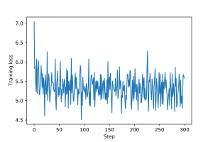
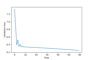
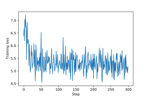
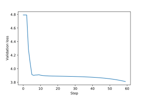
An example of training loop for this graph filter, including epochs and validation and test steps, is provided here. Plots for the training and validation loss are shown in Figures 1 and 2.

3.1 Graph Perceptron

Graph neural networks (GNNs) extend graph filters by using pointwise nonlinearities which are nonlinear functions that are applied independently to each component of a vector. For a formal definition, begin by introducing a single variable function $\sigma:\reals\to\reals$ which we extend to the vector function $\sigma:\reals^{n}\to\reals^{n}$ by independent application to each component. Thus, if we have $\bbu = [u_1, \ldots, u_{n}] \in \reals^{n}$ the output vector $\sigma(\bbu)$ is such that

\begin{equation} \label{eqn_ch8_pointwise_nonlinearity}
\sigma\big(\,\bbu\,\big) \ : \ \big[\,\sigma\big(\,\bbu\,\big)\,\big]_i = \sigma\big(\,u_i\,\big).
\end{equation}

I.e., the output vector is of the form $\sigma(\bbu) = [\sigma(u_1), \ldots, \sigma(u_{n})]$. Observe that we are abusing notation and using $\sigma$ to denote both the scalar function and the pointwise vector function.

In a single layer GNN, the graph signal $\bbu = \bbH(\bbS)\bbx$ is passed through a pointwise nonlinear function satisfying \eqref{eqn_ch8_pointwise_nonlinearity} to produce the output

\begin{equation} \label{eqn:graphPerceptron}
\bbPhi(\bbx;\bbh, \bbS) = \sigma(\bbu) = \sigma(\bbH(\bbS)\bbx) = \sigma \left( \sum_{k=0}^{K-1} \bbS^k \bbx h_k \right) \ .
\end{equation}

We say that the transform in \eqref{eqn:graphPerceptron} is a graph perceptron. Different from the graph filter in \eqref{eqn:graphFilter}, the graph perceptron is a nonlinear function of the input. It is, however, a very simple form of nonlinear processing because the nonlinearity does not mix signal components. Signal components are mixed by the graph filter but are then processed element-wise through $\sigma$.

To implement a graph perceptron, we simply modify the $\p{GraphFilter}$ module to take a generic nonlinearity $\p{sigma}$ as an input parameter:

class GraphPerceptron(nn.Module):
    def __init__(self, gso, k, sigma):
        super().__init__()
        self.gso = torch.tensor(gso)
        self.n = gso.shape[0]
        self.k = k
        self.sigma = sigma
        self.weight = nn.Parameter(torch.randn(self.k))
        self.reset_parameters()
        
    def reset_parameters(self):
        stdv = 1. / math.sqrt(self.k)
        self.weight.data.uniform_(-stdv, stdv)

    def forward(self, x):
        y = FilterFunction(self.weight, self.gso, x)
        y = self.sigma(y)
        return y    

To instantiate a graph perceptron with $K=8$ and ReLU nonlinearity, simply invoke:

graphPerceptron = GraphPerceptron(S, 8, nn.ReLU())

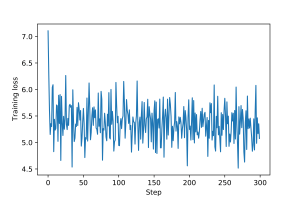
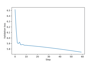
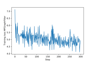
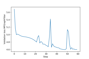
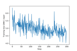
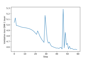
An example of training loop for this graph perceptron is provided here. The training and validation loss plots for the graph perceptron are shown in Figures 3 and 4.

3.2 Multi-layer GNN

Graph perceptrons can be stacked in layers to create multi-layer GNNs. This stacking is mathematically written as a function composition where the outputs of a layer become inputs to the next layer. For a formal definition let $\ell=1,\ldots,L$ be a layer index and $\bbh_\ell=\{h_{\ell k}\}_{k=0}^{K-1}$ be collections of $K$ graph filter coefficients associated with each layer. Each of these sets of coefficients define a respective graph filter $\bbPhi (\bbx; \bbh_\ell, \bbS) = \sum_{k=0}^{K-1} \bbS^k\bbx h_{\ell k}$. At layer $\ell$ we take as input the output $\bbx_{\ell-1}$ of layer $\ell-1$ which we process with the filter $\bbPhi (\bbx; \bbh_\ell, \bbS)$ to produce the intermediate feature

\begin{align}\label{eqn_ch8_gnn_recursion_single_feature_filter}
\bbu_{\ell} \ = \ \bbH_\ell(\bbS)\, \bbx_{\ell-1}
\ = \ \sum_{k=0}^{K-1} \bbS^k\, \bbx_{\ell-1} h_{\ell k},
\end{align}

where, by convention, we say that $\bbx_0 = \bbx$ so that the given graph signal $\bbx$ is the GNN input. As in the case of the graph perceptron, this feature is passed through a pointwise nonlinear function to produce the $\ell$th layer output

\begin{align}\label{eqn:mlGraphPerceptron}
\bbx_{\ell} \ = \ \sigma(\bbu_\ell )
\ = \ \sigma\Bigg(\sum_{k=0}^{K-1} \bbS^k\, \bbx_{l-1} h_{\ell k}\Bigg) .
\end{align}

After recursive repetition of \eqref{eqn_ch8_gnn_recursion_single_feature_filter}-\eqref{eqn:mlGraphPerceptron} for $\ell=1,\ldots,L$ we reach the $L$th layer whose output $\bbx_L$ is not further processed and is declared the GNN output $\bby=\bbx_L$. To represent the output of the GNN we define the filter tensor $\bbH:=\{\bbh_\ell\}_{\ell=1}^L$ grouping the $L$ sets of filter coefficients at each layer, and define the operator $\bbPhi(\,\cdot\,;\bbH,\bbS)$ as the map

\begin{align}\label{eqn_ch8_gnn_operator_single_feature}
\bbPhi (\bbx; \bbH, \bbS) = \bbx_L.
\end{align}

We repeat that in \eqref{eqn_ch8_gnn_operator_single_feature} the GNN output $\bbPhi (\bbx; \bbH, \bbS) = \bbx_L$ follows from recursive application of \eqref{eqn_ch8_gnn_recursion_single_feature_filter}-\eqref{eqn:mlGraphPerceptron} for $\ell=1,\ldots,L$ with $\bbx_0=\bbx$. Observe that this operator notation emphasizes that the output of a GNN depends on the filter tensor $\bbH$ and the graph shift operator $\bbS$.

We also emphasize that, similar to the case of the graph filters in \eqref{eqn:graphFilter}, the optimization is over the filter tensor $\bbH$ with the shift operator $\bbS$ given.

In PyTorch, a multi-layer GNN can be built using the $\p{graphPerceptron}$ module. Specifically, we implement a $\p{torch.nn.Module}$ that takes in the GSO, the number of layers, the number of filter taps in each layer and the nonlinearity and instantiates as many perceptrons as there are layers:

class MLGNN(nn.Module):
    def __init__(self, gso, l, k, sigma):
        super().__init__()
        layers = []
        for layer in range(l):
            layers.append(GraphPerceptron(gso, k[layer], sigma))
        self.layers = nn.Sequential(*layers)

    def forward(self, x):
        y = self.layers(x)
        return y

Note that $\p{k}$ is now a list of integers (as opposed to a single integer) with length equal to the number of layers, and that $\p{nn.Sequential}$ transforms a list of $\p{nn.Modules}$ into a layered architecture. To instantiate a multi-layer GNN with $K_1=8$ and $K_2=1$ from this class, invoke:

MLGNN = MLGNN(S, 2, [8, 1], nn.ReLU())

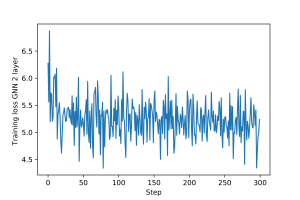
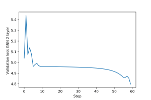
An example of training loop for the multi-layer GNN is provided here. The training and validation loss plots for the multi-layer GNN are shown in Figures 5 and 6.

4.1-4.3 Multiple Feature Filters and GNNs

To further increase the representation power of multi-layer GNNs, we incorporate multiple features per layer that are the result of processing multiple input features with a bank of graph filters.
Let $F_{in}$ be the number of input features and $F_{out}$ be the number of output features. Define the feature matrix $\bbX \in \reals^{N \times F_{in}}$ as

\begin{equation}
\bbX = [\bbx^1, \bbx^2, \ldots , \bbx^{F_{in}}].
\end{equation}

We have that $\bbX \in\reals^{N \times F_{in}}$ and interpret each column of $\bbX$ as a graph signal. For a compact representation of a filterbank made up of $F_{in}\times F_{out}$ filters, consider coefficient matrices $\bbH_{k}\in\reals^{F_{in}\times F_{out}}$. The filterbank is defined as

\begin{align}\label{eqn:filterBank}
\bbPhi(\bbX;\bbH,\bbS) \ = \ \sum_{k=0}^{K-1} \bbS^k\, \bbX\, \bbH_{k}
\end{align}

where the tensor $\bbH$ groups the filter coefficients $\bbH_k$, $\bbH = \{\bbH_{k}\}_{k}$.

To implement a multi-feature graph filter in PyTorch, we update the function $\p{FilterFunction}$ and the class $\p{GraphFilter}$ as follows:

def FilterFunction(h, S, x):
    
    # Number of output features
    F = h.shape[0]
    
    # Number of filter taps
    K = h.shape[1]
    
    # Number of input features
    G = h.shape[2]
    
    # Number of nodes
    N = S.shape[1]
    
    # Batch size
    B = x.shape[0]

    # Create concatenation dimension and initialize concatenation tensor z
    x = x.reshape([B, 1, G, N])
    S = S.reshape([1, N, N])
    z = x
    
    # Loop over the number of filter taps
    for k in range(1, K):
        
        # S*x
        x = torch.matmul(x, S)
        
        # Reshape
        xS = x.reshape([B, 1, G, N])
        
        # Concatenate
        z = torch.cat((z, xS), dim=1)
    
    # Multiply by h
    y = torch.matmul(z.permute(0, 3, 1, 2).reshape([B, N, K*G]), 
                     h.reshape([F, K*G]).permute(1, 0)).permute(0, 2, 1)
    return y
    
    
class GraphFilter(nn.Module):
    def __init__(self, gso, k, f_in, f_out):
        super().__init__()
        self.gso = torch.tensor(gso)
        self.n = gso.shape[0]
        self.k = k
        self.f_in = f_in
        self.f_out = f_out
        self.weight = nn.Parameter(torch.randn(self.f_out, self.k, self.f_in))
        self.reset_parameters()
        
    def reset_parameters(self):
        stdv = 1. / math.sqrt(self.f_in * self.k)
        self.weight.data.uniform_(-stdv, stdv)

    def forward(self, x):
        return FilterFunction(self.weight, self.gso, x)

Note that we assume that the input signal $\p{x}$ is a PyTorch tensor with shape $\p{[B,G,N]}$, where $\p{B}$ is the batch or data size, $\p{G}$ is the number of input features and $\p{N}$ is the number of nodes. The output signal tensor has shape $\p{[B,F,N]}$, where $\p{F}$ is the number of output features.

Using the updated $\p{GraphFilter}$ module, we instantiate a $2$-layer graph filter with $F_1=32$, $K_1=8$ and $K_2=1$ by using $\p{torch.nn.Sequential}$ to stack two multi-feature graph filters:

GraphFilter = torch.nnSequential(GraphFilter(gso=S, k=8, f_in=1, f_out=32),GraphFilter(gso=G, k=1, f_in=32, f_out=1))

Observe that the input features of the first filter and the output features of the second are set to $1$.

In their most general form, GNNs consist of compositions of filter banks as in \eqref{eqn:filterBank} with pointwise nonlinearities $\sigma$. Explicitly, let $F_\ell$ be the number of features at layer $\ell$ and define the feature matrix $\bbX_\ell$ as

\begin{equation}
\bbX_\ell = [\bbx_\ell^1, \bbx_\ell^2, \ldots , \bbx_\ell^{F_\ell}]\text{.}
\end{equation}

We have that $\bbX_\ell\in\reals^{N\times F_\ell}$ where each column is a graph signal. The outputs of layer $\ell-1$ are inputs to layer $\ell$ where the set of $F_{\ell-1}$ features in $\bbX_{\ell-1}$ are processed by a filterbank made up of $F_{\ell-1}\times F_\ell$ filters (cf. \eqref{eqn:filterBank}) to obtain the intermediate feature matrix

\begin{align}\label{eqn_ch8_gnn_recursion_filter_matrix}
\bbU_{\ell} \ = \ \sum_{k=0}^{K-1} \bbS^k\, \bbX_{\ell-1}\, \bbH_{ \ell k} \ .
\end{align}

As in the case of the single feature GNN (cf. \eqref{eqn:mlGraphPerceptron}) — and the graph perceptron in \eqref{eqn:graphPerceptron} — the intermediate feature $\bbU_{\ell}$ is passed through a pointwise nonlinearity to produce the $\ell$th layer output

\begin{align}\label{eqn:gnn}
\bbX_{\ell} \ = \ \sigma(\bbU_{\ell} )
\ = \ \sigma\Bigg(\sum_{k=0}^{K-1} \bbS^k\, \bbX_{\ell-1}\, \bbH_{\ell k} \Bigg).
\end{align}

When $\ell=0$ we convene that $\bbX_0=\bbX$ is the input to the GNN which is made of $F_0$ graph signals. The output $\bbX_L$ of layer $L$ is also the output of the GNN which is made up of $F_L$ graph signals. To define a GNN operator we group filter coefficients $\bbH_{\ell k}$ in the tensor $\bbH = \{\bbH_{\ell k}\}_{\ell ,k}$ and define the GNN operator

\begin{align}\label{eqn_ch8_gnn_operator_multifeature}
\bbPhi (\bbX; \bbH, \bbS) = \bbX_L.
\end{align}

If the input is a single graph signal as in \eqref{eqn:graphPerceptron} and \eqref{eqn_ch8_gnn_operator_single_feature}, we have $F_0=1$ and $\bbX_0=\bbx\in\reals^n$. If the output is also a single graph signal — as is also the case in \eqref{eqn:graphPerceptron} and \eqref{eqn_ch8_gnn_operator_single_feature} — we have $F_L=1$ and $\bbX_L=\bbx_L\in\reals^N$.

The multi-feature GNN module is implemented analogously to the multi-layer GNN from 3.2, i.e., by alternating graph filters (which are now multi-feature) and nonlinear pointwise activation functions. Explicitly,

class GNN(nn.Module):
    def __init__(self, gso, l, k, f, sigma):
        super().__init__()
        self.gso = torch.tensor(gso)
        self.n = gso.shape[0]
        self.l = l
        self.k = k
        self.f = f
        self.sigma = sigma
        
        gml = []
        for layer in range(l):
            gml.append(GraphFilter(gso,k[layer],f[layer],f[layer+1]))
            gml.append(sigma)
        
        self.gml = nn.Sequential(*gml)
        
    def forward(self, x):
        return self.gml(x)

Note that the input arguments $\p{k}$ and $\p{f}$ are both lists enumerating the number of filter taps and features of each layer. The length of the list $\p{f}$ is always equal to the number of layers $\p{l}$ plus one, as the number of features of the input data has to be specified as the first element of $\p{f}$.

To instantiate the 2-layer GNN from 4.2, invoke:

GNN2ly = GNN(gso=S, l=2, k=[8,1], f=[1,32,1], sigma=nn.ReLU())

Similarly, instantiate the 3-layer GNN from 4.3 by invoking:

GNN3ly = GNN(gso=S, l=3, k=[5,5,1], f=[1,16,4,1], sigma=nn.ReLU())

An example of training loop for the $2$-layer multi-feature graph filter from 4.1, as well as for the two GNNs above, is provided here. The training and validation loss plots for each architecture are shown in Figures 7-12.

5.1-5.3 Generalization

We went over linear and nonlinear graph parametrizations of the learning model $\bbPhi(\bbx; \ccalH)$, but there are several other possible choices of parametrization. For instance, we could choose $\bbPhi(\bbx; \ccalH)$ to be a simple linear transform (i.e., a $N \times N$ matrix) or a fully connected neural network (FCNN). This raises the question of why we favor graph filters, and even more so GNNs, over linear transforms and FCNNs. We answer this question by comparing five architectures: a generic linear transform, a FCNN, a graph filter and two GNNs.

The generic linear transform is implemented using the PyTorch class $\p{torch.nn.Linear}$:

linearParam = torch.nn.Linear(N, N)

Similarly, we implement the fully connected by stacking a linear layer, a nonlinearity, and another linear layer and nonlinearity using $\p{torch.nn.Sequential}$:

fcNet = nn.Sequential(torch.nn.Linear(N, 25), nn.ReLU(), torch.nn.Linear(25, N), nn.ReLU())

These architectures are then compared with the multi-layer filterbank and the GNNs from 4.1-4.3. A full training loop for all five architectures can be found here. Since $\p{torch.nn.Linear}$ layers have built-in bias, we have modified our $\p{FilterFunction}$, $\p{GraphFilter}$ and $\p{GNN}$ classes to include it (we also found that adding bias terms makes training more stable). Our results are shown in the table below.

	Linear	FCNN	Graph Filter	GNN 1yr	GNN 2 lyr	Min. GNNs
Mean	5.50	5.82	5.03	4.94	5.81	4.88
Median	5.42	5.71	4.96	4.89	5.51	4.83
Std	0.41	0.42	0.36	0.37	0.89	0.30

Note that the graph filter and the 1-layer GNN do better than the linear parametrization and the FCNN. Also note that the 1-layer GNN performs better than the graph filter. The 2-layer GNN seems to diverge; however, observe that the minimum loss achieved by both GNNs is even smaller, on average, than the loss achieved by the graph filter.

In your solution, you may have found that the GNNs don’t always work better than the graph filter due to divergences in training. This can happen, as GNNs are not always guaranteed to converge. To avoid this problem, make sure to select graph and dataset realizations for which the training loss does not diverge. You can use plots like the ones in items 2.3-4.3 to monitor the evolution of the training loss.

5.4-5.7 Transferability

In order to adapt the GNN model to be able to change the GSO, we first need to adapt the graph filters that compose its layers. This is done by adding the method $\p{changeGSO}$ to the $\p{GraphFilter}$ module of item 4.1:

class GraphFilter(nn.Module):
    def __init__(self, gso, k, f_in, f_out, bias):
        super().__init__()
        self.gso = torch.tensor(gso)
        self.n = gso.shape[0]
        self.k = k
        self.f_in = f_in
        self.f_out = f_out
        if bias:
            self.bias = nn.parameter.Parameter(torch.Tensor(self.f_out, 1))
        self.weight = nn.Parameter(torch.randn(self.f_out, self.k, self.f_in))
        self.reset_parameters()
        
    def reset_parameters(self):
        stdv = 1. / math.sqrt(self.f_in * self.k)
        self.weight.data.uniform_(-stdv, stdv)
        
        if self.bias is not None:
            self.bias.data.uniform_(-stdv, stdv)

    def forward(self, x):
        return FilterFunction(self.weight, self.gso, x, self.bias)
    
    def changeGSO(self, new_gso):
        self.gso = torch.tensor(new_gso)
        self.n = new_gso.shape[0]

We can then add a $\p{changeGSO}$ method to the $\p{GNN}$ module which calls the method above for every layer:

class GNN(nn.Module):
    def __init__(self, gso, l, k, f, sigma, bias):
        super().__init__()
        self.gso = torch.tensor(gso)
        self.n = gso.shape[0]
        self.l = l
        self.k = k
        self.f = f
        self.sigma = sigma
        self.bias = bias
        
        gml = []
        for layer in range(l):
            gml.append(GraphFilter(gso,k[layer],f[layer],f[layer+1], bias))
            gml.append(sigma)
        
        self.gml = nn.Sequential(*gml)
        
    def forward(self, x):
        return self.gml(x)
    
     def changeGSO(self, new_gso):
        self.gso = new_gso
        for layer in range(2*self.l):
            if layer
                self.gml[layer].changeGSO(new_gso)
        self.n = new_gso.shape[0] 

After repeating steps 1.1 and 1.2 for $N_2=500$, you should have the GSO of the new graph $\p{S2}$ and the test data $\p{(xTest2, yTest2)}$. To change the GSO of the saved GNN models and test them on this data, simply invoke:

GNN2ly.changeGSO(S2)
GNN3ly.changeGSO(S2)

with torch.no_grad():
    yHatTest2 = GNN2ly(xTest2)
lossTest2_GNN2ly= loss(yHatTest2, yTest2)

with torch.no_grad():
    yHatTest2 = GNN3ly(xTest2)
lossTest2_GNN3ly= loss(yHatTest2, yTest2)

Finally, you can solve 5.7 by repeating the steps above for $N_3=1000$. A full training loop with the solutions to all items in Section 5 can be found here, and our transferability results are shown in the table below:

	N=50	N=500	N=1000
1 lyr	5.68	6.01	6.17
2 lyr	5.39	6.15	6.34

Note that the RMSE differences are relatively small in all cases. For the 1-layer GNN, the relative RMSE differences are 5.9% and 8.7% respectively. For the 2-layer GNN, they are 14.2% and 17.7%. We will see that, in general, shallow and narrow GNNs transfer better than deeper and wider ones.