Lab 5: Distributed Collaborative Systems (11/20 – 12/6)
Graph neural networks (GNNs) explore the irregular structure of graph signals, and exhibit superior performance in various applications of recommendation systems, wireless networks and control. A key property GNNs inherit from graph filters is the distributed implementation. This property makes them suitable candidates for distributed learning over large-scale networks, where global information is not available at individual agents. Each agent must decide its own actions from local observations and communication with immediate neighbors. In this lab assignment, we focus on the distributed learning with graph neural networks.
1 Distributed Control Systems
We consider a team of $N$ agents tasked with controlling a dynamical process that is evolving in the space where the team is deployed. The system is distributed because the agents are located in different positions. We characterize this dynamical process by the collection of state values $\bbx_{i}(t)\in\reals^p$ as well as the collection of
control actions $\bbu_{i}(t)\in\reals^q$ that agents take. In this notation, $i$ represents an agent index and $t$ represents continuous time. We further group local states and local actions into matrices $\bbX(t) = [\bbx_{1}(t), \ldots, \bbx_{N}(t)]^{T}\in\reals^{N\times p}$ and $\bbU(t) = [\bbu_{1}(t), \ldots, \bbu_{N}(t)]^{T}\in\reals^{N\times q}$ that represent the global state of the system and the global control action at time $t$. Observe that row $n$ of $\bbX(t)$ is the state associated with agent $n$ and that row $n$ of $\bbU(t)$ is the control action taken by agent $n$.
With these definitions we write the evolution of the dynamical process through a differential equation of the form,
\begin{equation} \label{eq:continuousDynamic}
\dot{\bbX}(t) = f\Big(\bbX(t), \bbU(t)\Big) .
\end{equation}
In order to design a controller for this dynamical system we operate in discrete time by introducing a sampling time $T_s$ and a discrete time index $n$. We define $\bbX_{n} = \bbX(nT_s)$ as the discrete time state and $\bbU_{n}$ as the control action held from time $nT_s$ until time $(n+1)T_s$. Solving the differential equation between times $nT_s$ and $(n+1)T_s$, we end up with the discrete dynamical system
\begin{equation} \label{eq:discreteDynamic}
\bbX_{n+1} =
\bbX_n +
\int_{nT_s}^{(n+1)T_s}
f \Big(\bbX(t),\bbU_{n}\Big)\,\ dt ,
\qquad
\text{with~} \bbX(nT_s) = \bbX_{n} .
\end{equation}
At each point in (discrete) time, we consider a cost function $c(\bbX_n, \bbU_n)$. The objective of the control system is to choose actions $\bbU_n$ that reduce the accumulated cost $\sum_{n=0}^\infty c(\bbX_n, \bbU_n)$.
When the collection of state observations $\bbX_{n} = [\bbx_{1n}^{T};\ldots;\bbx_{Nn}^{T}]$ is available at a central location it is possible for us to consider centralized policies $\Pi$ that choose control actions $\bbU_n = \Pi(\bbX_n)$ that depend on global information. In such case the optimal policy is the one that minimizes the expected long term cost.
\begin{equation} \label{eq:optimalController}
\Pi^*_{\text{C}} = \underset{\Pi}{\mathrm{argmin}}
\mbE\Bigg[\sum_{n=0}^\infty c \Big(\bbX_n, \Pi(\bbX_n) \Big) \Bigg].
\end{equation}
If the dynamics in $f(\bbX(t),\bbU(t))$ and the costs $c \big( \bbX_n, \bbU_n \big)$ are known, as we assume here, there are several techniques to find the optimal policy $\Pi^*$. Our interest in this exercise is in decentralized controllers that operate without access to global information. In those situations, implementing \eqref{eq:optimalController} is not possible because of delays in percolating information through the distributed system.
2 Network Consensus
To ground the discussion we consider a consensus problem. The goal of a consensus problem is to compute an average over a network. It is not a difficult problem. In fact, one would venture that it is elementary. Yet, the solution in a decentralized setting becomes complicated. It, therefore, serves as a good illustration of the challenges of decentralized control.
To be more specific consider a reference velocity $\bbr_{n} = \bbr(nT_s)\in\reals^2$. This reference velocity evolves according to a random acceleration model that we write in discrete time as
\begin{equation}\label{eqn_consensus_reference}
\bbr_{n+1} = \bbr_{n} + T_s \Delta\bbr_{n}.
\end{equation}
In \eqref{eqn_consensus_reference}, the acceleration term $\Delta\bbr_{in}$ is white Gaussian with independent components and expected norm $\mbE(|\Delta\bbr_{n}|)$[1] # Hyperparameters (hParams) for the Local GNN hParamsLocalGNN['name'] = 'LocalGNN' hParamsLocalGNN['archit'] = modules.LocalGNN_DB hParamsLocalGNN['device'] = 'cuda:0' \ if (True and torch.cuda.is_available()) \ else 'cpu' hParamsLocalGNN['dimNodeSignals'] = [6, 64] # Features per layer hParamsLocalGNN['nFilterTaps'] = [4] # Number of filter taps hParamsLocalGNN['bias'] = True hParamsLocalGNN['nonlinearity'] = nn.Tanh hParamsLocalGNN['dimReadout'] = [2] hParamsLocalGNN['dimEdgeFeatures'] = 1 if torch.cuda.is_available(): torch.cuda.empty_cache() hParamsDict = deepcopy(hParamsLocalGNN) thisName = hParamsDict.pop('name') callArchit = hParamsDict.pop('archit') thisDevice = hParamsDict.pop('device') ############## # PARAMETERS # ############## thisArchit = callArchit(**hParamsDict) thisArchit.to(thisDevice) thisOptim = optim.Adam(thisArchit.parameters(), lr = learningRate, betas = (beta1, beta2)) thisLossFunction = nn.MSELoss() thisTrainer = training.TrainerFlocking GraphNNs = model.Model(thisArchit, thisLossFunction, thisOptim, thisTrainer, thisDevice, thisName, saveDir) #Train GraphNNs.train(simulator, positions, ref_vel, est_vel, est_vels, biased_vels, accels, networkss, nEpochs, batchSize) #Test ref_vel_test = ref_vel[200:220] est_vel_test = est_vel[200:220] pos_test = positions[200:220] _, _, est_vels_valid, biased_vels_valid, accels_valid = simulator.computeTrajectory_pos_collision(GraphNNs.archit, pos_test, ref_vel_test, est_vel_test, 100) cost = simulator.cost(est_vels_valid, biased_vels_valid, accels_valid) print(cost)
Finally, we can plot the relevant graphs for this experiment.
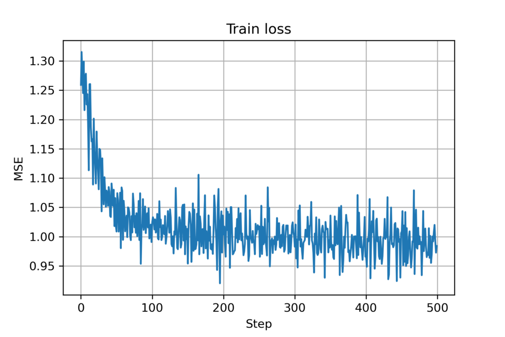
Figure 9. Training loss for GNN (with mobility and collision avoidance)
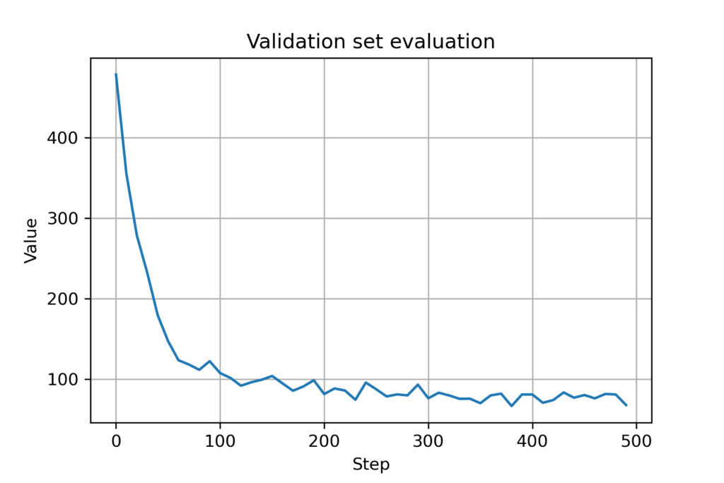
Figure 10. Validation cost for GNN (with mobility and collision avoidance)
As we did before with the centralized and decentralized controller, we can plot the average velocity difference for a number of trajectories.
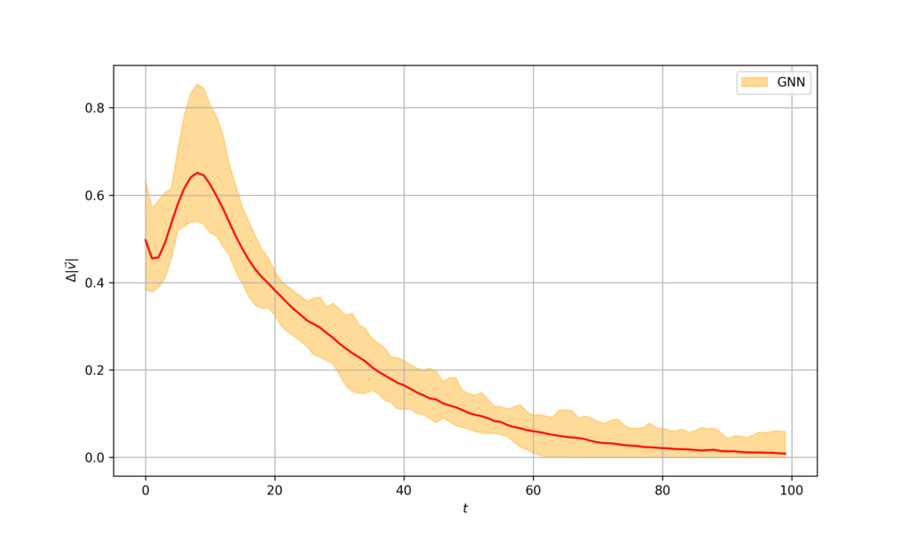
Figure 11. Velocity difference for GNN controller
As it can be seen, it performs significantly better than the decentralized controller that we developed previously. This can be seen by directly comparing it with the centralized and the decentralized controllers.
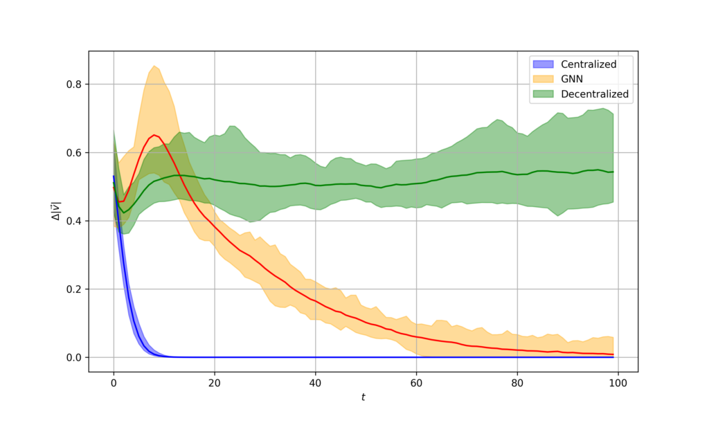
Figure 12. Velocity difference for comparison (centralized, decentralized, and GNN controller)
As we did before, we can also plot the individual velocities – observe that while it takes a longer period than with the centralized controller, the velocities do converge at one point.
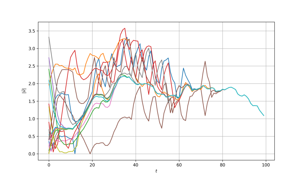
Figure 13. Velocity evolution for GNN controller
As an additional illustration, we can see how our controller performs by plotting the trajectories for the $N$ agents:
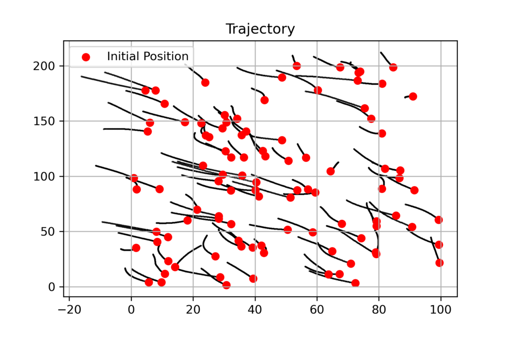
Figure 14. Representative trajectory for GNN controller
- A Gaussian random variable $X$ in two dimensions with independent components, each of which has variance $\sigma^2$, has a expected norm $\mbE(|X|) = \sigma\sqrt{\pi/2}$. To generate a Gaussian with expected norm $\mbE(|X|)$ we use variances $\sigma^2 = (2/\pi)\mbE^2(|X|)$ in each component.}. The initial reference velocity $\bbr_{0}$ is initialized with a normal distribution with zero mean independent components and expected norm $\mbE(|\bbr_{0}|)$.
We consider a team of $n$ agents whose goal is to estimate this reference velocity. However, the agents do not observe the reference directly. Each of them observes a biased version of the reference velocity according to the model
\begin{equation}\label{eqn_consensus_observations}
\bbr_{in} = \bbr_{n} + \Delta\bbr_{i}.
\end{equation}The bias terms $\Delta\bbr_{i}$ of each agent are white Gaussian with independent components and expected norm $\mbE(|\Delta\bbr_{i}|)$. Notice that the bias term does not change over time. It is a systematic error in the velocity measurements of each agent.
The reference velocities in \eqref{eqn_consensus_observations} are observations of agents. In addition to this observations, agents have velocity estimates $v_{in}$. These velocities evolve according to the dynamical model
\begin{equation}\label{eqn_consensus_dynamics}
\bbv_{i(n+1)} = \bbv_{in} + T_s \bbu_{in},
\end{equation}
in which $\bbu_{in}$ is a control acceleration that is to be chosen by agent $i$. The goal of the agents is to make this estimate as close as possible to the reference velocity $\bbr_{n}$. This velocity, however, is not observed by the team. We therefore set to find a policy that controls for the cost function
\begin{equation}\label{eqn_consensus_cost_centralized_no_aceleration}
\tdc(\bbV_n, \bbR_n) =
\frac{1}{2N}
\sum_{i=1}^N
\left | \,
\bbv_{in} – \frac{1}{N}\sum_{j=1}^N \bbr_{jn}
\, \right|^2.
\end{equation}
According to \eqref{eqn_consensus_cost_centralized_no_aceleration}, the goal is for each agent to find out velocities $\bbv_{in}$ that coincide with the average reference velocity $(1/N)\sum_{j=1}^N \bbr_{jn}$ observed by the team. If it helps to fix ideas, you can think of a flock that wants to move with the wind. They each observe the wind with some systematic error and collaborate to follow the average of their wind estimates.To minimize the cost in \eqref{eqn_consensus_cost_centralized_no_aceleration} we just need to get the swarm to follow the average. Namely, to make $\bbv_{in} = (1/N\sum_{j=1}^N \bbr_{jn})$. To make the problem more interesting we ask for a balance between velocity reduction and energy. The latter depends on the acceleration $\bbu_{in}$. We therefore consider a relative weight $\lambda$ and define the cost
\begin{equation}\label{eqn_consensus_cost_centralized}
c(\bbV_n, \bbR_n, \bbU_n) =
\frac{1}{2N}
\sum_{i=1}^N
\left | \,
\bbv_{in} – \frac{1}{N}\sum_{j=1}^N \bbr_{jn}
\, \right|^2
+
\frac{\lambda}{2N}
\sum_{i=1}^N\Big| \, T_s\bbu_{in} \, \Big|^2 \, .
\end{equation}
In the general problem definition we consider the cost over a time horizon [cf. \eqref{eq:optimalController}]. To keep the problem simple we consider here a greedy formulation where at time step $n$ we want to minimize the cost $c(\bbV_{n+1}, \bbR_{n+1}, \bbU_{n+1})$ at the next time step. This result in a simple expression for the optimal control policy in which the acceleration of agent $i$ is given by
\begin{equation}\label{eqn_consensus_optimal_policy_centralized}
\bbu_{in}^*
= \frac{-1}{T_s(1+\lam)}
\left ( \,
\bbv_{in} – \frac{1}{N}\sum_{j=1}^N \bbr_{jn}
\, \right) .
\end{equation}
The solution in \eqref{eqn_consensus_optimal_policy_centralized} computes the difference between the velocity of agent $i$ and the average reference velocity and accelerates in the opposite direction. The amount of acceleration is controlled by $\lambda$. The larger $\lambda$, the less we accelerate.In the following plots, we can see the performance of the centralized controller. As expected, the controller is able to reach a consensus on the velocities of the agents. Note that this controller assumes perfect knowledge over the whole network, which might not hold in practice.
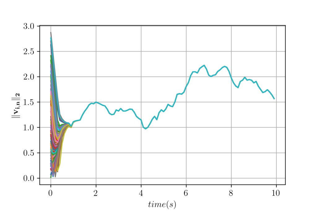
Figure 1. Velocity trajectories of 100 agents. 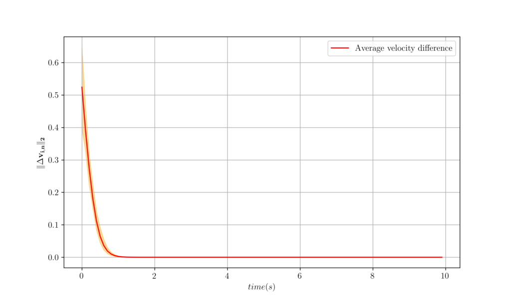
Figure 2. The worst, best, and Average velocity difference over 100 agents. The yellow region represent the area between the best and worst cases. 2.1 Decentralized Consensus
The consensus problem we have just described becomes more interesting when formulated in a distributed setting. To do that, assume that agents are connected through a communication network. The network is described by a set of edges $(i,j)\in\ccalE_n$ which induce the neighborhoods $\ccalN_{in}$. With a graph restricting the exchange of information, the implementation of \eqref{eqn_consensus_optimal_policy_centralized} becomes impossible.
An important point to repeat is that it becomes difficult to design appropriate controllers. Our goal is still the minimization of the cost in \eqref{eqn_consensus_cost_centralized} but this is difficult to do with the partial information we are given. Faced with the impossibility of finding optimal controllers, we can resort to approximations. A natural idea is to forget about the fact that information is delayed and just evaluate \eqref{eqn_consensus_optimal_policy_centralized} with the information we have. We therefore define the averages
\begin{equation}\label{eqn_consensus_neighborhood_averages}
\bar\bbr_{jn}^k
= \frac{1}{\#\left(\ccalN_{in}^k\right)}
\sum_{j\in\ccalN_{in}^k} \bbr_{j (n-k)} ,
\end{equation}which represent the average velocity of the $k$-hop neighbors of node $i$ corrected by appropriated delays. Using these averages we can now approximate the controller in \eqref{eqn_consensus_optimal_policy_centralized} as
\begin{equation}\label{eqn_consensus_dcentralized_policy}
\bbu_{in}^\dagger
= \frac{-1}{T_s(1+\lam)}
( \,
\bbv_{in} – \frac{1}{K}\sum_{k=1}^K \bar\bbr_{jn}^k
\, ) .
\end{equation}The controller defined by \eqref{eqn_consensus_neighborhood_averages} and \eqref{eqn_consensus_dcentralized_policy} is decentralized because it respects the information history structure. The values that are needed for implementing \eqref{eqn_consensus_dcentralized_policy} are available at node $i$ because they have been relayed through neighbors. That the controller can be implemented does not mean it will be any good. We are taking averages of out of date information.
The fact that we are referring to $\bbv_{in}$ as the velocity of agent $i$ at time $n$ hints at moving agents. We are going to go there in the last section, but for the time being we are neglecting the fact that agents are moving. This is important because as agents move the communication network changes. This is not an issue except that it increases the cost of your simulation due the the necessity to recompute the communication graph.
In the following plots, we can see the performance of the decentralized controller. It can be see that the decentralized controller fails to achieve velocity consensus in the network. This is even the case when we utilize information from $K$-hop neighbors. The fact that this controller does not attain a good performance is because, the data is delayed one step for each one hop and we average over outdated data. You can play around and try to design your own controller, by weighting differently the contributions from different hop neighbors. Instead of doing so, in the next section we will learn the controller from the data.
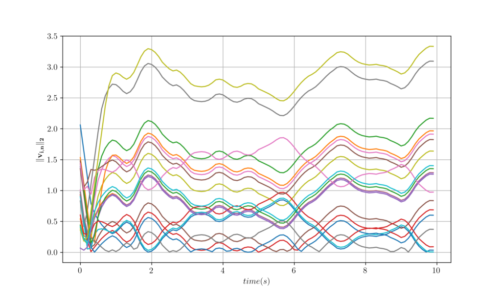
Figure 3. Velocity trajectories of 20 agents with K = 4 and D = 2. 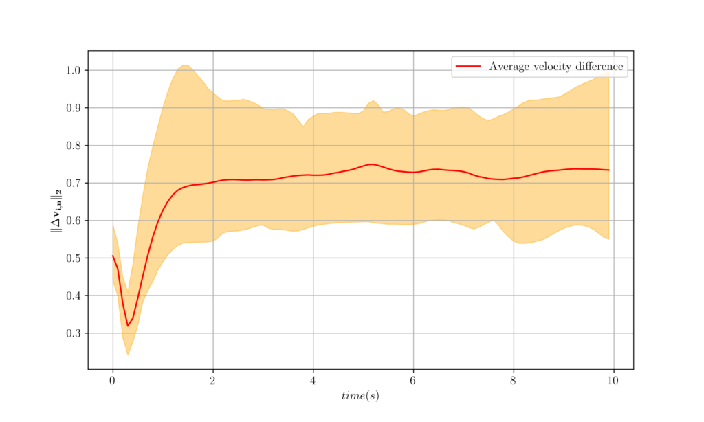
Figure 4. The worst, best and average velocity difference over 100 agents attained from a decentralized controller. 3 Learning Distributed Controllers
In Section 2 we explained the inherent complexity of decentralized control. In Section 2.1 we illustrated that these inherent complexities lead to important differences in practical performance. One can attribute the performance penalty to the fact that \eqref{eqn_consensus_dcentralized_policy} forgets the fact that it is averaging information that can be out of date. This is true, but how can we correct for that? Say we choose to discount older information. This is a sensible idea but how do we choose discount factors? The problem is not that decentralized control becomes impossible to solve. But since finding the optimal controller is impossible, we are left to choose among many possible heuristics.
If we are settling for heuristics, there is no reason to overlook the use of learned heuristics. We use our models as a source of simulated data and fit a learned parametrization. This is the idea we described in Section2. The goal of mimicking the optimal centralized policy means that, at least in principle, the learned heuristic can learn an optimal controller. This is something we give away in designed heuristics.
If we decide to settle for learned heuristics, our job as system designers is not complete. We should still choose the parametrization. Since we are considering a problem where a network plays a central role, the choice of parametrization is clear: We should choose graph filters and graph neural networks (GNNs). In the case of distributed systems there is a second, more important reason for us to use graph filters and GNNs: They can be implemented in a distributed manner while respecting the information structure of distributed control.
3.1 Distributed Implementation of Graph Filters and GNNs
To explain the use of graph filters and GNNs in distributed systems we start by recalling our definition of MIMO graph filters as polynomials on the graph shift operator $\bbS$.
\begin{equation}\label{eqn_graph_filter_conventional}
\bbZ = \sum_{k=0}^K \bbS^k \bbX \bbH_k .
\end{equation}In the case of distributed systems the matrix graph signal $\bbX$ is evolving over time index $n$. We therefore introduce a time varying version of \eqref{eqn_graph_filter_conventional} in which the $k$th term of the polynomial multiplies the signal $\bbX_{n-k}$
\begin{equation}\label{eqn_graph_filter_modified}
\bbZ_n = \sum_{k=0}^K\bbS^k \bbX_{n-k} \bbH_k .
\end{equation}The reason for introducing this modification in \eqref{eqn_graph_filter_modified} is that it is now possible to provide a distributed implementation that respects the information history structure from the agents available neighborhood. To see how this is done we express \eqref{eqn_graph_filter_modified} in terms of a modified diffusion sequence. This diffusion sequence is initialized as $\bbY_{n0} = \bbX_n$ and its subsequent elements are computed recursively as
\begin{equation}\label{eqn_diffusion_sequence}
\bbY_{nk} = \bbS \bbY_{(n-1)(k-1)}.
\end{equation}Applying this definition recursively we have that $\bbY_{nk} = \bbS^k \bbY_{(n-k)0}$. Further recalling the initialization condition we have that $\bbY_{(n-k)0} = \bbX_{n-k}$. Thus, $\bbY_{nk} = \bbS^k \bbX_{n-k}$ and we have that the the filter in \eqref{eqn_graph_filter_modified} can be equivalently written as a summation of elements of the diffusion sequence,
\begin{equation}\label{eqn_graph_filter_difussion}
\bbZ_n = \sum_{k=0}^K \bbY_{nk}\bbH_k
\end{equation}To show that we can implement \eqref{eqn_graph_filter_difussion} in a distributed manner, it suffices if we show that each of the $\bbY_{nk}$ terms can be evaluated through local computation exchanges. To see that this is true recall that the shift operator shares the sparsity pattern of the graph. Thus, when we look at the computation of the $i$th entry of $\bbY_{nk}$ we can write
\begin{equation}\label{eqn_diffusion_local}
\Big[\,\bbY_{nk}\,\Big]{i} = \sum{j\in \ccalN_{ni}}
\Big[\,\bbS \,\Big]{ij} \times \Big[\, \bbY{(n-1)(k-1)} \,\Big]_{j} \,.
\end{equation}According to \eqref{eqn_diffusion_local}, node $i$ can compute the $i$th entry of $\bbY_{nk}$ if it receives information from neighboring agents $j$ about the values of the $j$th entries of the $\bbY_{(n-1)(k-1)}$. This is something that is available to node $i$ because it can be communicated from its neighboring agents $j$. These are, by definition, the agents with which $i$ can communicate.
If a graph filter can be implemented in a distributed manner, a GNN can be as well. This is because the nonlinearity is pointwise and can be implemented locally. Having seen that a GNN can respect the information structure of distributed systems, we can use them as learning parametrizations in decentralized control. This is the goal of the next question.
In the following plots we can see that GNNs close the gap between centralized controllers that cannot be implemented in practice and decentralized controllers. GNNs work because they learn the relationships between hops in the network, and are stable to perturbations and equivariant to relabeling. These two last properties will be studied in the next two sections.
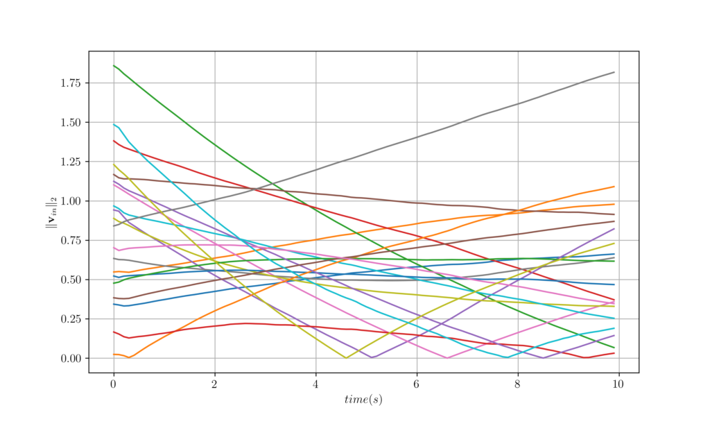
Figure 5. Velocity trajectories of 20 agents over time for question 3.1. 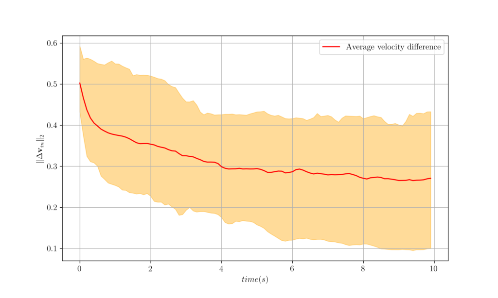
Figure 6. The worst, best and average velocity difference over 100 agents attained from GNNs. 4 Agent Mobility
In this section, we modify the problem in to incorporate agent mobility. Denote as $\bbp_{in}$ the position of agent $i$ at time $n$ and augment the dynamical model in \eqref{eqn_consensus_dynamics} to incorporate the dynamics that control this variable,
\begin{equation}\label{eqn_position_dynamics}
\bbp_{i(n+1)} = \bbp_{in} + T_s \bbv_{in} + (T_s^2/2) \bbu_{in}.
\end{equation}When we incorporate agent mobility the first aspect of the problem that changes is that the network is no longer fixed. As agents move, their set of nearest neighbors change. This is consistent with our generic problem description . To make our graph filters consistent with a time varying network we just need to modify the definition of the diffusion sequence to take time varying networks into consideration. We thus replace \eqref{eqn_graph_filter_modified} by $ \bbY_{nk} = \bbS_n \bbY_{(n-1)(k-1)}$ where $\bbS_n$ is the shift operator of the communication network at time $n$.
In this part of the lab we are going to run a GNN not trained considering the position, on a network of agents whose communication network varies as time passes. In the following plot we can see that the GNN that is agnostic to the position is able to control the agents.
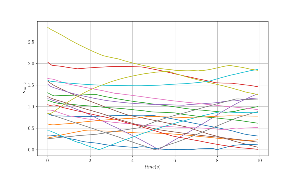
Figure 7. Velocity trajectories of 20 agents over time for question 4.1. 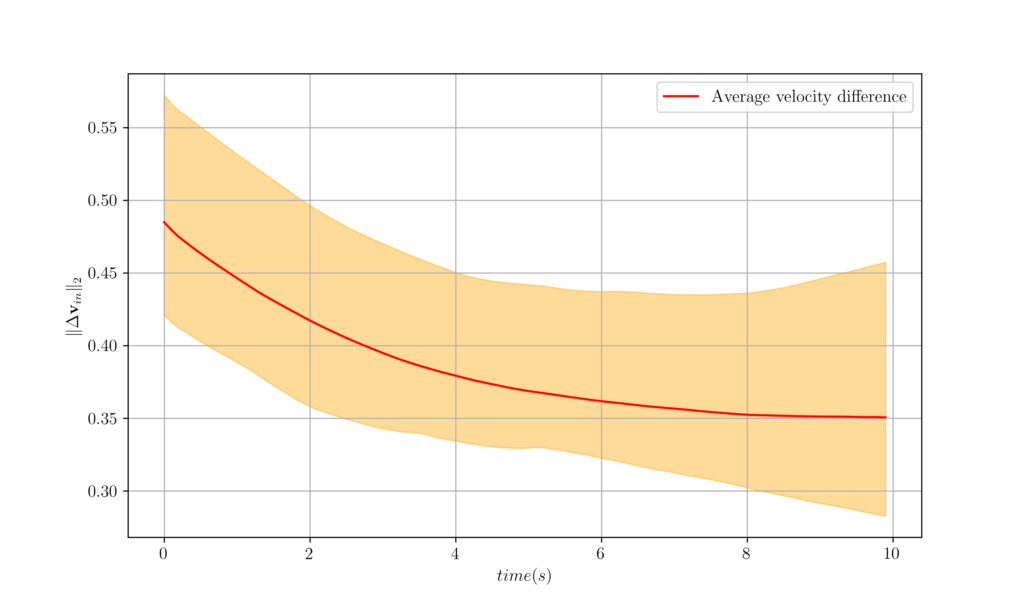
Figure 8. The worst, best and average velocity difference over 100 agents attained from GNNs trained on fixed graphs and tested over time-varying graphs. This came as no surprise as we know that GNNs are stable, in fact we have studied several types of stability in Lectures 6 and 7. In this experiment, we can see the manifestation of the stability properties of GNNs, as even though the graph changes, the GNN is able to control the agents.
Now, we can train a GNN considering the position of the agents. We will see that as positions can be expressed as a graph signal, the GNN will exploit its structure.
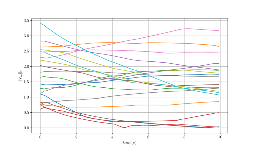
Figure 9. Velocity trajectories of 20 agents over time for question 4.3. 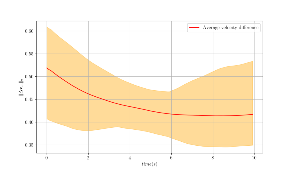
Figure 10. The worst, best and average velocity difference over 100 agents attained from GNNs trained and tested over time-varying graphs. It is important to now stop and think how to derive the decentralized controller in this setting. It is not trivial to allocate different weights accounting for different distances, and velocities, let alone accounting for delayed information in the graph. This makes GNNs even more valuable.
5 Collision and Spread Avoidance
The second aspect of the problem that changes when we incorporate mobility is that agents can get too close to each other, which would result in a collision. Agents can also get too far apart, which would result in their inability to communicate. To prevent both outcomes we utilize a potential function to encourage neighboring agents to stay within a target distance of each other. Formally, let $\bbp_{in}$ be the position of agent $i$ at time $n$ and $\bbp_{jn}$ be the position of agent $j$. Agents $j$ is a neighbor of agent $i$. We then define the potential
\begin{equation}\label{eqn_potential}
U( \bbp_{in}, \bbp_{jn} )
= \frac{d_0^2}{| \bbp_{in} -\bbp_{jn} |^2}
+ \log\left[ \frac{| \bbp_{in} -\bbp_{jn} |^2}{d_0^2}\right]
\end{equation}This potential function has a minimum when the distance between agents $i$ and $j$ is $| \bbp_{in} -\bbp_{jn} |^2 = d_0$.
The potentials $U( \bbp_{in}, \bbp_{jn} )$ in \eqref{eqn_potential} are added to the cost function in \eqref{eqn_consensus_cost_centralized} to define the loss function
\begin{equation}\label{eqn_cost_mobility}
\ell(\bbP_n, \bbV_n, \bbR_n, \bbU_n)
= c(\bbV_n, \bbR_n, \bbU_n) +
\frac{\mu}{2N}
\sum_{i=1}^N
\frac{1}{\#\left(\ccalN_{in}\right)}
\sum_{j\in\ccalN_{in}}
U( \bbp_{in}, \bbp_{jn} ) .
\end{equation}
The optimal centralized controller is the one that greedily minimizes the cost in \eqref{eqn_cost_mobility} at each time step. Our goal in this section is to learn a GNN controller that mimics this optimal centralized controller.Before we set out to design this GNN, we define the following feature at node $i$,
\begin{equation}\label{eqn_mobility_feature}
\bbq_{in}
= \frac{1}{\#\left(\ccalN_{in}\right)}
\sum_{j\in\ccalN_{in}}
\bbp_{in}, \bbp_{jn} .
\end{equation}
This is the center of mass of the neighbors of $i$ measured relative to the position of node $i$. In this definition, it is not very important that $\bbq_{in}$ be a center of mass. But is is very important that the measure be relative so as to preserve permutation equivariance. This is because GNNs are equivariant to node relabeling, and thus if we consider distances measured relative to the node, we can leverage the properties of the GNN. This translates into signals that will require the same output independent of which node is being considered, only the distance to its neighbors carries valuable information for avoiding collisions.Now we are going to learn a distributed policy that mimics the optimal centralized controller that minimizes the cost in \eqref{eqn_cost_mobility} with a GNN. The input features to the GNN are $\bbV_n$, $\bbR_n,$ and $\bbQ_n$.
Here we can see that the GNN works well on a decentralized setting. It is important to note that albiet controllers can be obtained for the easy setting of consensus, as more information and requirements are added, the controllers become computationally costly and difficult to obtain. Besides, as we have seen in section 3, they not always work in practice.
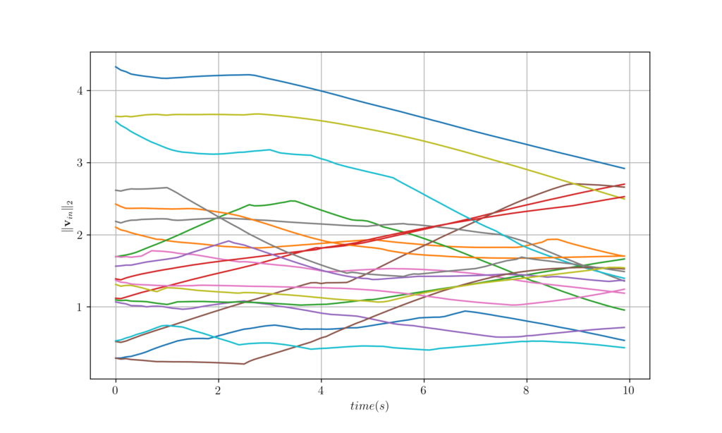
Figure 11. Velocity trajectories of 20 agents over time for question 5.2. 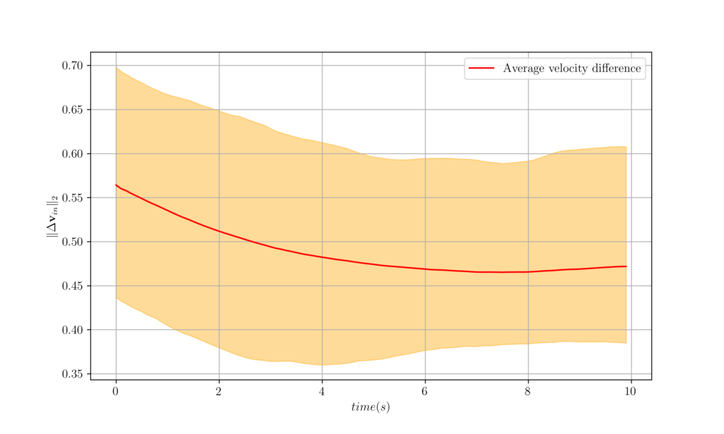
Figure 12. The worst, best and average velocity difference over 100 agents. 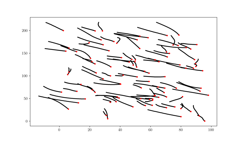
Figure 13. Position trajectories of 100 agents over time. The red points show the staring position of each agent. 6 Code
The code can be found here. An in-depth explanation of how to obtained the code can be found below.
To simulate the system described by (12)-(14), we create the file $\p{consensus}$ that contains the Python class $\p{ConsensusSimulator}$ as. It contains the function $\p{simulate}$ that actually computes the entire simulation for the system; note that this function takes in an argument $\p{controller}$ which is responsible for effectively controlling the agents (i.e. determining the acceleration) at each time step.
from abc import ABC
import torch
import numpy as np

class ConsensusSimulator:
    def __init__(
            self,
            N,
	    nSamples,
            initial_ref_vel=1.0,
            ref_vel_delta=1.0,
            ref_vel_bias=4.0,
	    ref_est_delta=1.0,
            max_agent_acceleration=3.0,
            sample_time=0.1,
	    duration=10,
            energy_weight=1,
            is_bias_constant=True
    ):
        self.N = N
        self.nSamples = nSamples
        self.initial_ref_vel = initial_ref_vel
        self.ref_vel_delta = ref_vel_delta
        self.ref_vel_bias = ref_vel_bias
        self.ref_est_delta = ref_est_delta
        self.max_agent_acceleration = max_agent_acceleration
        self.sample_time = sample_time
        self.tSamples = int(duration / self.sample_time)
        self.energy_weight = energy_weight
        self.is_bias_constant = is_bias_constant

    def random_vector(self, expected_norm, N, samples):
        return np.random.normal(0, (2 / 3.14) ** 0.5 * expected_norm, (samples, 2, N))

    def bias(self):
        return self.random_vector(self.ref_vel_bias, self.N, self.nSamples)

    def initial(self):
        ref_vel = self.random_vector(self.initial_ref_vel, 1, self.nSamples)
        est_vel = ref_vel + self.random_vector(self.ref_est_delta, self.N, self.nSamples)
        return ref_vel, est_vel

    def simulate(self, steps, controller: ConsensusController):

        ref_vel, est_vel = self.initial()
        bias = self.bias()

        ref_vels = np.zeros((self.nSamples, self.tSamples, 2, 1))
        est_vels = np.zeros((self.nSamples, self.tSamples, 2, self.N))
        biased_vels = np.zeros((self.nSamples, self.tSamples, 2, self.N))
        accels = np.zeros((self.nSamples, self.tSamples, 2, self.N))

        ref_vels[:,0,:,:] = ref_vel
        est_vels[:,0,:,:] = est_vel
        biased_vels[:,0,:,:] = bias + ref_vel
        accels[:,0,:,:] = controller(est_vels, biased_vels, 0)

        this_accel = accels[:,0,:,:].copy()
        this_accel[accels[:,0,:,:] > self.max_agent_acceleration] = self.max_agent_acceleration
        this_accel[accels[:,0,:,:] < -self.max_agent_acceleration] = -self.max_agent_acceleration
        accels[:,0,:,:] = this_accel

        for step in range(1, steps):

            ref_accel = self.random_vector(self.ref_vel_delta, 1, self.nSamples)
            ref_vels[:,step,:,:] = ref_vels[:,step-1,:,:] + ref_accel * self.sample_time
            est_vels[:,step,:,:] = accels[:,step-1,:,:] * self.sample_time + est_vels[:,step-1,:,:]
            biased_vels[:,step,:,:] = bias + ref_vels[:,step,:,:]

            accels[:,step,:,:] = controller(est_vels, biased_vels, step)

            this_accel = accels[:,step,:,:].copy()
            this_accel[accels[:,step,:,:] > self.max_agent_acceleration] = self.max_agent_acceleration
            this_accel[accels[:,step,:,:] < -self.max_agent_acceleration] = -self.max_agent_acceleration
            accels[:,step,:,:] = this_accel

        return ref_vel, est_vel, est_vels, biased_vels, accels

    def cost(self, est_vels, biased_vels, accels):

        biased_vel_mean = np.mean(biased_vels, axis = 3)
        biased_vel_mean = np.expand_dims(biased_vel_mean, 3)
        vel_error = est_vels - biased_vel_mean
        vel_error_norm = np.square(np.linalg.norm(vel_error, ord=2, axis=2, keepdims=False))
        vel_error_norm_mean = np.sum(np.mean(vel_error_norm, axis = 2), axis = 1)

        accel_norm = np.square(np.linalg.norm(self.sample_time * accels, ord=2, axis=2, keepdims=False))
        accel_norm_mean = np.sum(np.mean(accel_norm, axis = 2), axis = 1)

        cost = np.mean(vel_error_norm_mean/2 + accel_norm_mean/2)

        return cost
2.2 Optimal controller
To implement the optimal controller, we create the python class $\p{Optimal Controller}$ in the file $\p{consensus}$ as:
class ConsensusController(ABC):
    def __call__(self, est_vel, biased_vel):
        pass

class OptimalController(ConsensusController):
    def __init__(self, sample_time=0.1, energy_weight=1):
        self.sample_time = sample_time
        self.energy_weight = energy_weight

    def __call__(self, est_vel, biased_vel, step):

        mean_biased_vel  = np.mean(biased_vel[:,step,:,:], axis=2)
        mean_biased_vel = np.expand_dims(mean_biased_vel, 2)

        return -(est_vel[:,step,:,:] - mean_biased_vel) / (self.sample_time * (1 + self.energy_weight))
Running the simulation with $N=100$ and $T = 10$, we observe that the average velocity of the agents quickly converge. We can see this by plotting the velocity difference at each time step.
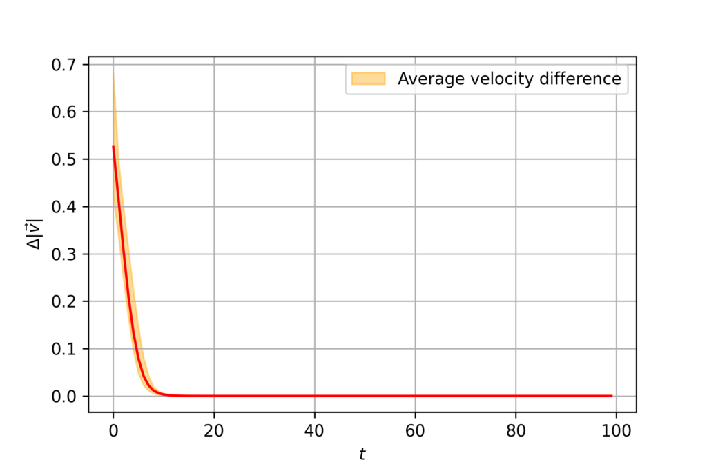
Figure 1. Velocity difference for centralized controller
We can also plot individual velocity evolution so we see how it progresses through time. Note that they converge with time.
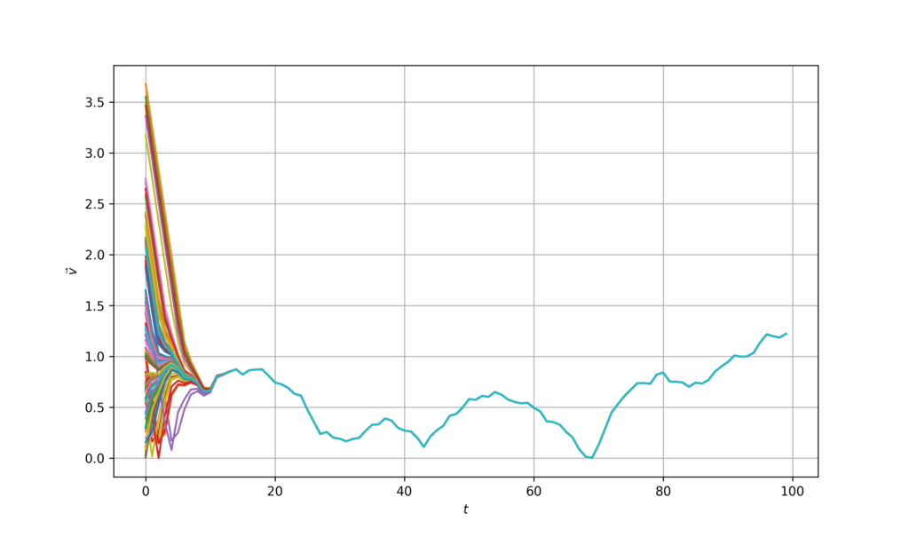
Figure 2. Velocity evolution for centralized controller
2.3 Communication network
To implement the decentralized controller, we first create the file $\p{networks}$ to create the function that computes the communication graph – the graph shift operator $\mathbf{S}$. This function returns both the regular communication graph and a normalized version.
import numpy as np
from scipy.spatial import distance_matrix
import copy
import heapq
rng = np.random

def agent_communication(wx, wy, n_agents, degree):
    positions = np.vstack((
        rng.uniform(0, wx, n_agents),
        rng.uniform(0, wy, n_agents)))
    distance = distance_matrix(positions.T, positions.T)
    network = copy.deepcopy(distance)
    for i in range(n_agents):
        re2 = heapq.nsmallest((degree+1), distance[i,:])
        for j in range(n_agents):
            if distance[i,j] > re2[degree]:
                network[i,j] = 0
    network = network + np.transpose(network, axes = [1,0])
    network[np.arange(0,n_agents),np.arange(0,n_agents)] = 0.
    network = (network > 0).astype(distance.dtype)
    W = np.linalg.eigvalsh(network)
    maxEigenvalue = np.max(np.real(W))
    normalized_network = network / maxEigenvalue

    return network, normalized_network
2.4 Decentralized controller
With the communication network available, we then create the python class $\p{DistributedController}$ for decentralized controller in the file $\p{consensus}$ as:
class DistributedController(ConsensusController):
    def __init__(self, adjacency, K=1, sample_time=0.1, energy_weight=1):

        self.nSamples = adjacency.shape[0]
        self.nAgents = adjacency.shape[1]
        self.K = K
        self.neighbor_network = np.zeros((self.nSamples, K, self.nAgents, self.nAgents))
        self.num_neighbor = np.zeros((self.nSamples, K, 2, self.nAgents))

        for i in range(self.nSamples):
            for k in range(1, (K+1)):
                inter_matrix = np.linalg.matrix_power(adjacency[i,:,:], k)
                inter_matrix[inter_matrix>=1] = 1
                self.num_neighbor[i,k-1,0,:] = np.sum(inter_matrix,1)
                self.num_neighbor[i,k-1,1,:] = np.sum(inter_matrix,1)
                self.neighbor_network[i,k-1,:,:] = inter_matrix

        self.sample_time = sample_time
        self.energy_weight = energy_weight

    def __call__(self, est_vel, biased_vel, step):
        # find the averages along 0,K neighborhoods and average them
        biased_means = np.zeros((self.nSamples, self.K, 2, self.nAgents))

        if step < (self.K-1):
            for k in range(step):
                biased_means[:,k,:,:] = np.matmul(biased_vel[:,step-k,:,:], self.neighbor_network[:,k,:,:])
                biased_means[:,k,:,:] = biased_means[:,k,:,:] / self.num_neighbor[:,k,:,:]
        else:
            for k in range(self.K):
                biased_means[:,k,:,:] = np.matmul(biased_vel[:,step-k,:,:], self.neighbor_network[:,k,:,:])
                biased_means[:,k,:,:] = biased_means[:,k,:,:] / self.num_neighbor[:,k,:,:]
        biased_mean = np.mean(biased_means, 1)
        return (biased_mean - est_vel[:,step,:,:]) / (self.sample_time * (1 + self.energy_weight))
Together, we use above classes to perform system simulations in the file $\p{main}$ as:
from importlib import reload
import numpy as np
import consensus
import networks
consensus = reload(consensus)
networks = reload(networks)

#
D = 2
K = 1
nSamples = 200
N = 100

com_network = np.zeros((nSamples, N, N))

#
for i in range(nSamples):
    com_network[i,:,:], _ = networks.agent_communication(100, 200, N, D)

#
optimal_controller = consensus.OptimalController()
decentralized_controller = consensus.DistributedController(com_network, K)
simulator = consensus.ConsensusSimulator(N, nSamples)

opt_ref_vel, opt_est_vel, opt_est_vels, opt_biased_vels, opt_accels = simulator.simulate(100, optimal_controller)
dec_ref_vel, dec_est_vel, dec_est_vels, dec_biased_vels, dec_accels = simulator.simulate(100, decentralized_controller)
opt_cost = simulator.cost(opt_est_vels, opt_biased_vels, opt_accels)
dec_cost = simulator.cost(dec_est_vels, dec_biased_vels, dec_accels)
Using the the code above, we can plot the average velocity difference as we did with the centralized controller. As one can observe, the velocity difference does not converge to zero in this case.
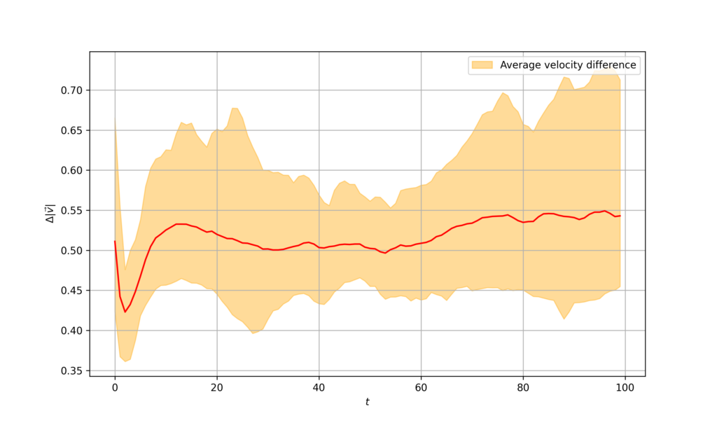 Figure 3. Velocity difference for decentralized controller
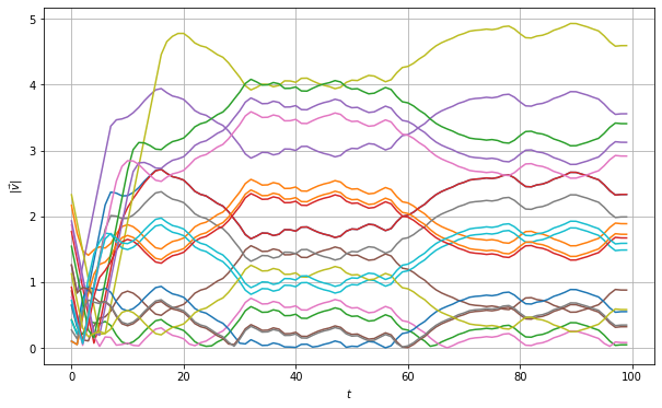
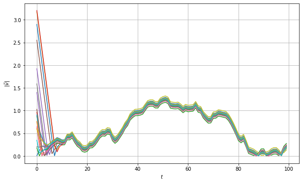
Figure 4. Velocity evolution for decentralized controller with K = 2
and K = 99 (respectively)3.1 Learning with a GNN
To learn a decentralized controller with a GNN, we will use $\p{LocalGNN_DB}$ GNN architecture based on the Alelab library.
class LocalGNN_DB(nn.Module):
    def __init__(self,
        dimNodeSignals, nFilterTaps, bias,
        nonlinearity,
        dimReadout,
        dimEdgeFeatures):
        super().__init__()
        self.L = len(nFilterTaps)
        self.F = dimNodeSignals
        self.K = nFilterTaps
        self.E = dimEdgeFeatures
        self.bias = bias
        self.sigma = nonlinearity
        self.dimReadout = dimReadout
        gfl0 = []
        for l in range(self.L):
            gfl0.append(GraphFilter_DB(self.F[l], self.F[l+1], self.K[l],
                self.E, self.bias))
            gfl0.append(self.sigma())
            self.GFL0 = nn.Sequential(*gfl0)
            fc0 = []
            if len(self.dimReadout) > 0:
                fc0.append(nn.Linear(self.F[-1], dimReadout[0], bias = self.bias))
                for l in range(len(dimReadout)-1):
                    fc0.append(self.sigma())
                    fc0.append(nn.Linear(dimReadout[l], dimReadout[l+1],
bias = self.bias))
            self.Readout0 = nn.Sequential(*fc0)
     def splitForward(self, x, S):
         assert len(S.shape) == 4 or len(S.shape) == 5
         if len(S.shape) == 4:
             S = S.unsqueeze(2)
         for l in range(self.L):
             self.GFL0[2*l].addGSO(S)
         yGFL0 = self.GFL0(x)
         y = yGFL0.permute(0, 1, 3, 2)
         y = self.Readout0(y)
         return y.permute(0, 1, 3, 2), yGFL0
         # B x T x dimReadout[-1] x N, B x T x dimFeatures[-1] x N
    def forward(self, x, S):
         output, _ = self.splitForward(x, S)
         return output
To perform the imitation learning, we need the validation to evaluate the cost in the training process. We create a function in the class $\p{ConsensusSimulator}$ (in the file $\p{consensus}$) named $\p{ComputeTrajectory}$ that simulates the trajectory by using the GNN controller for cost evaluation as:
import networks
import copy

    def computeTrajectory(self, archit, ref_vel, est_vel, step):

        batchSize = est_vel.shape[0]
        nAgents = est_vel.shape[2]
        ref_vel = ref_vel.squeeze(2)
        architDevice = list(archit.parameters())[0].device
        est_vels = np.zeros((batchSize, step, 2, nAgents), dtype = np.float)
        ref_vels = np.zeros((batchSize, step, 2), dtype = np.float)
        biased_ref_vels = np.zeros((batchSize, step, 2, nAgents), dtype = np.float)
        bias = np.zeros((batchSize, step, 2, nAgents))
        accels = np.zeros((batchSize, step, 2, nAgents), dtype=np.float)
        states = np.zeros((batchSize, step, 4, nAgents), dtype=np.float)
        graphs = np.zeros((batchSize, step, nAgents, nAgents), dtype = np.float)

        est_vels[:,0,:,:] = est_vel.copy()
        ref_vels[:,0,:] = ref_vel.copy()
        bias[:,0,:,:] = np.random.normal(loc=0,scale=(4 * np.sqrt(2/np.pi)),size=(batchSize, 2, nAgents))
        ref_vel_temp = np.expand_dims(ref_vels[:,0,:], 2)
        biased_ref_vels[:,0,:,:] = ref_vel_temp + bias[:,0,:,:]

        for i in range(20):
            _, graphs[i,0,:,:] = networks.agent_communication(100, 200, self.N, 2)

        for t in range(1, step):

            thisbiased_ref_vels = np.expand_dims(biased_ref_vels[:,t-1,:,:], 1)
            thisest_vels = np.expand_dims(est_vels[:,t-1,:,:], 1)
            thisState = np.concatenate((thisest_vels, thisbiased_ref_vels), axis = 2)
            states[:,t-1,:,:] = thisState.squeeze(1)

            x = torch.tensor(states[:,0:t,:,:], device = architDevice)
            S = torch.tensor(graphs[:,0:t,:,:], device = architDevice)
            with torch.no_grad():
                thisaccels = archit(x, S)
            thisaccels = thisaccels.cpu().numpy()[:,-1,:,:]
            thisaccels[thisaccels > 3] = 3
            thisaccels[thisaccels < -3] = -3
            accels[:,t-1,:,:] = thisaccels
            est_vels[:,t,:,:] = accels[:,t-1,:,:] * 0.1 +est_vels[:,t-1,:,:]
            ref_accel = np.random.normal(loc=0,scale=(self.ref_vel_delta * np.sqrt(2/np.pi)),size=(batchSize, 2))
            ref_vels[:,t,:] = ref_vels[:,t-1,:] + ref_accel * 0.1
            ref_vel_temp = np.expand_dims(ref_vels[:,t,:], 2)
            biased_ref_vels[:,t,:,:] = ref_vel_temp + bias[:,0,:,:]
            graphs[:,t,:,:] = copy.deepcopy(graphs[:,0,:,:])

        thisbiased_ref_vels = np.expand_dims(biased_ref_vels[:,-1,:,:], 1)
        thisest_vels = np.expand_dims(est_vels[:,-1,:,:], 1)
        thisState = np.concatenate((thisest_vels, thisbiased_ref_vels), axis = 2)
        states[:,-1,:,:] = thisState.squeeze(1)
        x = torch.tensor(states, device = architDevice)
        S = torch.tensor(graphs, device = architDevice)
        with torch.no_grad():
            thisaccels = archit(x, S)
        thisaccels = thisaccels.cpu().numpy()[:,-1,:,:]
        thisaccels[thisaccels > 3] = 3
        thisaccels[thisaccels < -3] = -3
        accels[:,-1,:,:] = thisaccels

        return ref_vel, est_vel, est_vels, biased_ref_vels, accels
We follow to build the imitation learning process for the GNN as the file $\p{training}$ (which inherits the Trainer class from the Alelab library):
import torch
import numpy as np
import datetime
class Trainer:
    def __init__(self, model, simulator, ref_vel, est_vel, est_vels, biased_vels, accels, S, nEpochs, batchSize):
        self.model = model
        self.est_vel = est_vel
        self.ref_vel = ref_vel
        self.est_vels = est_vels
        self.biased_vels = biased_vels
        self.accels = accels
        self.S = S
        self.nTrain = 200
        self.nTest = 20
        self.nValid = 20
        self.nEpochs = nEpochs
        self.simulator = simulator
        self.validationInterval = self.nTrain//batchSize
        if self.nTrain < batchSize:
           self.nBatches = 1
           self.batchSize = [self.nTrain]
        elif self.nTrain

class TrainerFlocking(Trainer):

    def __init__(self, model, simulator, ref_vel, est_vel, est_vels, biased_vels, accels, S, nEpochs, batchSize):

        super().__init__(model, simulator, ref_vel, est_vel, est_vels, biased_vels, accels, S, nEpochs, batchSize)

    def train(self):

        nTrain = self.nTrain
        thisArchit = self.model.archit
        thisLoss = self.model.loss
        thisOptim = self.model.optim
        thisDevice = self.model.device
        epoch = 0
        xTrainAll = np.concatenate((self.est_vels[0:self.nTrain].copy(), self.biased_vels[0:self.nTrain].copy()), axis = 2)
        yTrainAll = self.accels[0:self.nTrain].copy()
        StrainAll = self.S[0:self.nTrain].copy()

        while epoch < self.nEpochs:

            randomPermutation = np.random.permutation(nTrain)
            idxEpoch = [int(i) for i in randomPermutation]
            batch = 0

            while batch < self.nBatches:

                thisBatchIndices = idxEpoch[self.batchIndex[batch] : self.batchIndex[batch+1]]
                xTrain = xTrainAll[thisBatchIndices]
                yTrain = yTrainAll[thisBatchIndices]
                Strain = StrainAll[thisBatchIndices]

                xTrain = torch.tensor(xTrain, device = thisDevice)
                Strain = torch.tensor(Strain, device = thisDevice)
                yTrain = torch.tensor(yTrain, device = thisDevice)

                startTime = datetime.datetime.now()
                thisArchit.zero_grad()
                yHatTrain = thisArchit(xTrain, Strain)
                lossValueTrain = thisLoss(yHatTrain, yTrain)
                lossValueTrain.backward()
                thisOptim.step()
                endTime = datetime.datetime.now()
                timeElapsed = abs(endTime - startTime).total_seconds()
                del xTrain
                del Strain
                del yTrain
                del lossValueTrain

                #\\\\\\\
                #\\\ VALIDATION
                #\\\\\\\

                if (epoch * self.nBatches + batch)

                    startTime = datetime.datetime.now()
                    ref_vel = self.ref_vel[220:240]
                    est_vel = self.est_vel[220:240]
                    _, _, est_vels_valid, biased_vels_valid, accels_valid = self.simulator.computeTrajectory(thisArchit, ref_vel, est_vel, 100)
                    accValid = self.simulator.cost(est_vels_valid, biased_vels_valid, accels_valid)
                    endTime = datetime.datetime.now()
                    timeElapsed = abs(endTime - startTime).total_seconds()

                    print("\t(E:
                            epoch+1, batch+1,
                            accValid,
                            timeElapsed), end = ' ')
                    print("[VALIDATION] \n", end = '')

                    if epoch == 0 and batch == 0:
                        bestScore = accValid
                        bestEpoch, bestBatch = epoch, batch
                        self.model.save(label = 'Best')
                        # Start the counter
                    else:
                        thisValidScore = accValid
                        if thisValidScore < bestScore:
                            bestScore = thisValidScore
                            bestEpoch, bestBatch = epoch, batch
                            print("\t=> New best achieved:
                            self.model.save(label = 'Best')
                    del ref_vel
                    del est_vel
                batch += 1
            epoch += 1

        self.model.save(label = 'Last')
        #################
        # TRAINING OVER #
        #################
        if self.nEpochs == 0:
            self.model.save(label = 'Best')
            self.model.save(label = 'Last')
            print("\nWARNING: No training. Best and Last models are the same.\n")
        self.model.load(label = 'Best')
        if self.nEpochs > 0:
            print("\t=> Best validation achieved (E:
                    bestEpoch + 1, bestBatch + 1, bestScore))
and the file $\p{model}$ that contains the Python class $\p{Model}$ aggregating all training components with the GNN architecture (also available on the Alelab library).
import os
import torch

class Model:

    def __init__(self,
                 architecture,
                 loss,
                 optimizer,
                 trainer,
                 device, name, saveDir):

        self.archit = architecture
        self.nParameters = 0
        for param in list(self.archit.parameters()):
            if len(param.shape)>0:
                thisNParam = 1
                for p in range(len(param.shape)):
                    thisNParam *= param.shape[p]
                self.nParameters += thisNParam
            else:
                pass
        self.loss = loss
        self.optim = optimizer
        self.trainer = trainer
        self.device = device
        self.name = name
        self.saveDir = saveDir

    def train(self, simulator, ref_vel, est_vel, est_vels, biased_vels, accels, com_network, nEpochs, batchSize):

        self.trainer = self.trainer(self, simulator, ref_vel, est_vel, est_vels, biased_vels, accels, com_network, nEpochs, batchSize)

        return self.trainer.train()

    def save(self, label = '', **kwargs):
        if 'saveDir' in kwargs.keys():
            saveDir = kwargs['saveDir']
        else:
            saveDir = self.saveDir
        saveModelDir = os.path.join(saveDir,'savedModels')
        # Create directory savedModels if it doesn't exist yet:
        if not os.path.exists(saveModelDir):
            os.makedirs(saveModelDir)
        saveFile = os.path.join(saveModelDir, self.name)
        torch.save(self.archit.state_dict(), saveFile+'Archit'+ label+'.ckpt')
        torch.save(self.optim.state_dict(), saveFile+'Optim'+label+'.ckpt')

    def load(self, label = '', **kwargs):
        if 'loadFiles' in kwargs.keys():
            (architLoadFile, optimLoadFile) = kwargs['loadFiles']
        else:
            saveModelDir = os.path.join(self.saveDir,'savedModels')
            architLoadFile = os.path.join(saveModelDir,
                                          self.name + 'Archit' + label +'.ckpt')
            optimLoadFile = os.path.join(saveModelDir,
                                         self.name + 'Optim' + label + '.ckpt')
        self.archit.load_state_dict(torch.load(architLoadFile))
        self.optim.load_state_dict(torch.load(optimLoadFile))
We can then use aforementioned classes and files to train a decentralized GNN controller in the file $\p{main}$ as:
from importlib import reload
import numpy as np
import consensus
import networks
import os
import torch; torch.set_default_dtype(torch.float64)
import torch.nn as nn
import torch.optim as optim
import modules
import training
import model
import datetime
from copy import deepcopy

consensus = reload(consensus)
networks = reload(networks)

#
D = 2
K = 3
nSamples = 240
N = 100
step = 100

network = np.zeros((nSamples, N, N))
com_network = np.zeros((nSamples, step, N, N))

#
for i in range(nSamples):
    network[i,:,:], com_network[i,0,:,:] = networks.agent_communication(100, 200, N, D)
    for t in range(1, step):
        com_network[i,t,:,:] = deepcopy(com_network[i,0,:,:])

#
optimal_controller = consensus.OptimalController()
decentralized_controller = consensus.DistributedController(network, K)
simulator = consensus.ConsensusSimulator(N, nSamples)

ref_vel, est_vel, est_vels, biased_vels, accels = simulator.simulate(100, optimal_controller)

#
thisFilename = 'flockingGNN'
saveDirRoot = 'experiments'
saveDir = os.path.join(saveDirRoot, thisFilename)
today = datetime.datetime.now().strftime("
saveDir = saveDir + '-
# Create directory
if not os.path.exists(saveDir):
    os.makedirs(saveDir)

#   PyTorch seeds
torchState = torch.get_rng_state()
torchSeed = torch.initial_seed()
#   Numpy seeds
numpyState = np.random.RandomState().get_state()

nEpochs = 50 # Number of epochs
batchSize = 20 # Batch size
learningRate = 0.00025
beta1 = 0.9
beta2 = 0.999

hParamsLocalGNN = {} # Hyperparameters (hParams) for the Local GNN
hParamsLocalGNN['name'] = 'LocalGNN'
hParamsLocalGNN['archit'] = modules.LocalGNN_DB
hParamsLocalGNN['device'] = 'cuda:0' \
                                if (True and torch.cuda.is_available()) \
                                else 'cpu'
hParamsLocalGNN['dimNodeSignals'] = [4, 64] # Features per layer
hParamsLocalGNN['nFilterTaps'] = [4] # Number of filter taps
hParamsLocalGNN['bias'] = True
hParamsLocalGNN['nonlinearity'] = nn.Tanh
hParamsLocalGNN['dimReadout'] = [2]
hParamsLocalGNN['dimEdgeFeatures'] = 1

if torch.cuda.is_available():
    torch.cuda.empty_cache()
hParamsDict = deepcopy(hParamsLocalGNN)
thisName = hParamsDict.pop('name')
callArchit = hParamsDict.pop('archit')
thisDevice = hParamsDict.pop('device')

##############
# PARAMETERS #
##############

thisArchit = callArchit(**hParamsDict)
thisArchit.to(thisDevice)
thisOptim = optim.Adam(thisArchit.parameters(), lr = learningRate, betas = (beta1, beta2))
thisLossFunction = nn.MSELoss()
thisTrainer = training.TrainerFlocking
GraphNNs = model.Model(thisArchit, thisLossFunction, thisOptim, thisTrainer, thisDevice, thisName, saveDir)

#Train
GraphNNs.train(simulator, ref_vel, est_vel, est_vels, biased_vels, accels, com_network, nEpochs, batchSize)

#Test
ref_vel_test = ref_vel[200:220]
est_vel_test = est_vel[200:220]
_, _, est_vels_valid, biased_vels_valid, accels_valid = simulator.computeTrajectory(GraphNNs.archit, ref_vel_test, est_vel_test, 100)
cost = simulator.cost(est_vels_valid, biased_vels_valid, accels_valid)
print(cost)
The training loss plots and evaluation for the validation set are shown below.
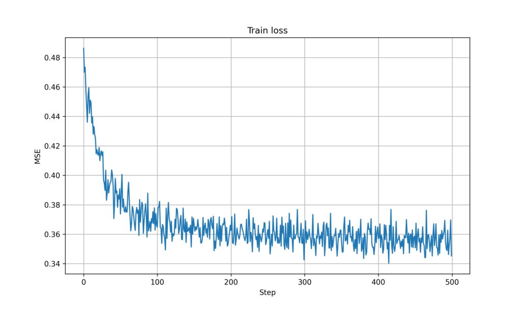
Figure 5. Training loss for GNN (no mobility)
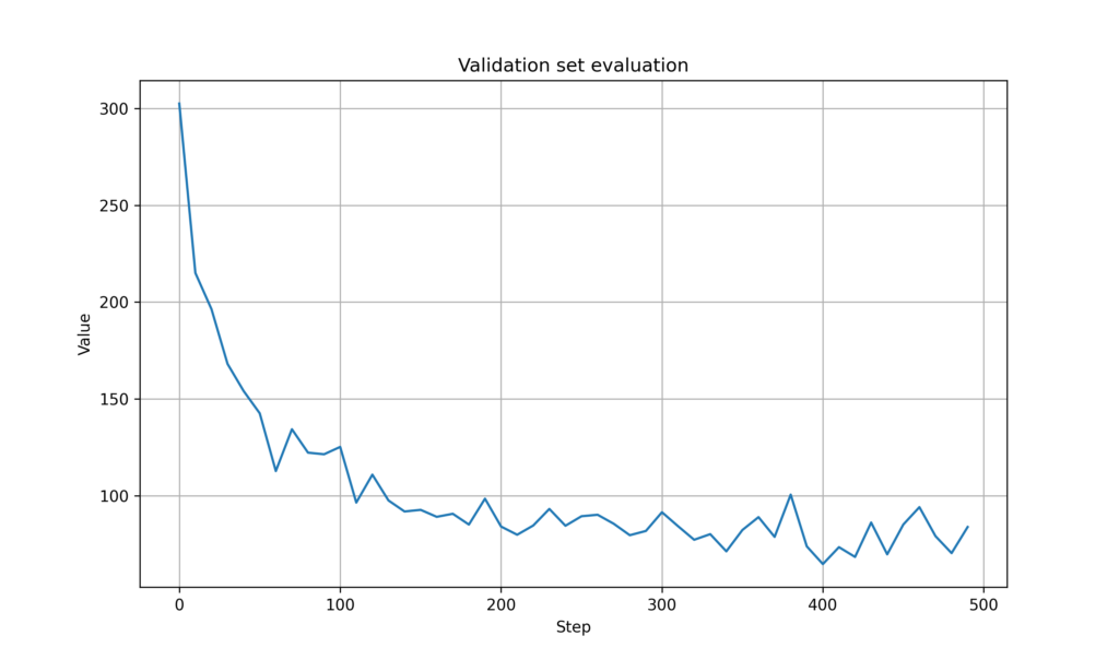
Figure 6. Validation cost for GNN (no mobility)
4.1-4.3 Agent Mobility
We proceed to account for the agent mobility. In this context, we first create the function in the file $\p{networks}$ that computes the communication graph based on agents positions as:
def agent_communication_pos(pos, n_agents, degree):

    distance = distance_matrix(pos.T, pos.T)
    network = copy.deepcopy(distance)
    for i in range(n_agents):
        re2 = heapq.nsmallest((degree+1), distance[i,:])
        for j in range(n_agents):
            if distance[i,j] > re2[degree]:
                network[i,j] = 0
    network = network + np.transpose(network, axes = [1,0])
    network[np.arange(0,n_agents),np.arange(0,n_agents)] = 0.
    network = (network > 0).astype(distance.dtype)
    W = np.linalg.eigvalsh(network)
    maxEigenvalue = np.max(np.real(W))
    normalized_network = network / maxEigenvalue

    return network, normalized_network
To consider agent mobility in the system simulation, we create the Python class $\p{simulatepos}$ in the class $\p{ConsensusSimulator}$ (in the file $\p{consensus}$) to incorporate communication graph changes induced by time-varying agent positions as:
    def simulate_pos(self, wx, wy, degree, steps, controller: ConsensusController):

        ref_vel, est_vel = self.initial()
        bias = self.bias()
        x_pos = np.random.uniform(0, wx, (self.nSamples, 1, self.N))
        y_pos = np.random.uniform(0, wy, (self.nSamples, 1, self.N))
        pos = np.concatenate((x_pos, y_pos), axis = 1)
        ref_vels = np.zeros((self.nSamples, self.tSamples, 2, 1))
        est_vels = np.zeros((self.nSamples, self.tSamples, 2, self.N))
        biased_vels = np.zeros((self.nSamples, self.tSamples, 2, self.N))
        accels = np.zeros((self.nSamples, self.tSamples, 2, self.N))
        positions = np.zeros((self.nSamples, self.tSamples, 2, self.N))
        networkss = np.zeros((self.nSamples, self.tSamples, self.N, self.N))
        ref_vels[:,0,:,:] = ref_vel
        est_vels[:,0,:,:] = est_vel
        biased_vels[:,0,:,:] = bias + ref_vel
        accels[:,0,:,:] = controller(est_vels, biased_vels, 0)
        positions[:,0,:,:] = pos
        for i in range(self.nSamples):
            _, networkss[i,0,:,:] = networks.agent_communication_pos(positions[i,0,:,:], self.N, degree)
        this_accel = accels[:,0,:,:].copy()
        this_accel[accels[:,0,:,:] > self.max_agent_acceleration] = self.max_agent_acceleration
        this_accel[accels[:,0,:,:] < -self.max_agent_acceleration] = -self.max_agent_acceleration
        accels[:,0,:,:] = this_accel

        for step in range(1, steps):
            ref_accel = self.random_vector(self.ref_vel_delta, 1, self.nSamples)
            ref_vels[:,step,:,:] = ref_vels[:,step-1,:,:] + ref_accel * self.sample_time
            est_vels[:,step,:,:] = accels[:,step-1,:,:] * self.sample_time + est_vels[:,step-1,:,:]
            positions[:,step,:,:] = accels[:,step-1,:,:] * (self.sample_time ** 2)/2 + est_vels[:,step-1,:,:] * self.sample_time + positions[:,step-1,:,:]
            for i in range(self.nSamples):
                _, networkss[i,step,:,:] = networks.agent_communication_pos(positions[i,step,:,:], self.N, degree)
            biased_vels[:,step,:,:] = bias + ref_vels[:,step,:,:]
            accels[:,step,:,:] = controller(est_vels, biased_vels, step)
            this_accel = accels[:,step,:,:].copy()
            this_accel[accels[:,step,:,:] > self.max_agent_acceleration] = self.max_agent_acceleration
            this_accel[accels[:,step,:,:] < -self.max_agent_acceleration] = -self.max_agent_acceleration
            accels[:,step,:,:] = this_accel

        return networkss, positions, ref_vel, est_vel, est_vels, biased_vels, accels
To evaluate the cost that accounts for agent mobility, we shall similarly create the Python function $\p{computeTrajectorypos}$ in the class $\p{ConsensusSimulator}$ (in the file $\p{consensus}$) as:
    def computeTrajectory_pos(self, archit, position, ref_vel, est_vel, step):

        batchSize = est_vel.shape[0]
        nAgents = est_vel.shape[2]
        ref_vel = ref_vel.squeeze(2)
        architDevice = list(archit.parameters())[0].device
        est_vels = np.zeros((batchSize, step, 2, nAgents), dtype = np.float)
        ref_vels = np.zeros((batchSize, step, 2), dtype = np.float)
        positions = np.zeros((batchSize, step, 2, nAgents), dtype = np.float)
        biased_ref_vels = np.zeros((batchSize, step, 2, nAgents), dtype = np.float)
        bias = np.zeros((batchSize, step, 2, nAgents))
        accels = np.zeros((batchSize, step, 2, nAgents), dtype=np.float)
        states = np.zeros((batchSize, step, 4, nAgents), dtype=np.float)
        graphs = np.zeros((batchSize, step, nAgents, nAgents), dtype = np.float)
        est_vels[:,0,:,:] = est_vel.copy()
        ref_vels[:,0,:] = ref_vel.copy()
        bias[:,0,:,:] = np.random.normal(loc=0,scale=(4 * np.sqrt(2/np.pi)),size=(batchSize, 2, nAgents))
        ref_vel_temp = np.expand_dims(ref_vels[:,0,:], 2)
        biased_ref_vels[:,0,:,:] = ref_vel_temp + bias[:,0,:,:]
        positions[:,0,:,:] = position[:,0,:,:]

        for i in range(20):
            _, graphs[i,0,:,:] = networks.agent_communication_pos(positions[i,0,:,:], nAgents, 2)

        for t in range(1, step):

            thisbiased_ref_vels = np.expand_dims(biased_ref_vels[:,t-1,:,:], 1)
            thisest_vels = np.expand_dims(est_vels[:,t-1,:,:], 1)
            thisState = np.concatenate((thisest_vels, thisbiased_ref_vels), axis = 2)
            states[:,t-1,:,:] = thisState.squeeze(1)

            x = torch.tensor(states[:,0:t,:,:], device = architDevice)
            S = torch.tensor(graphs[:,0:t,:,:], device = architDevice)
            with torch.no_grad():
                thisaccels = archit(x, S)
            thisaccels = thisaccels.cpu().numpy()[:,-1,:,:]
            thisaccels[thisaccels > 3] = 3
            thisaccels[thisaccels < -3] = -3
            accels[:,t-1,:,:] = thisaccels
            est_vels[:,t,:,:] = accels[:,t-1,:,:] * 0.1 +est_vels[:,t-1,:,:]
            positions[:,t,:,:] = accels[:,t-1,:,:] * (0.1 ** 2)/2 + est_vels[:,t-1,:,:] * 0.1 + positions[:,t-1,:,:]
            ref_accel = np.random.normal(loc=0,scale=(self.ref_vel_delta * np.sqrt(2/np.pi)),size=(batchSize, 2))
            ref_vels[:,t,:] = ref_vels[:,t-1,:] + ref_accel * 0.1
            ref_vel_temp = np.expand_dims(ref_vels[:,t,:], 2)
            biased_ref_vels[:,t,:,:] = ref_vel_temp + bias[:,0,:,:]
            for i in range(20):
                _, graphs[i,t,:,:] = networks.agent_communication_pos(positions[i,t,:,:], nAgents, 2)

        thisbiased_ref_vels = np.expand_dims(biased_ref_vels[:,-1,:,:], 1)
        thisest_vels = np.expand_dims(est_vels[:,-1,:,:], 1)
        thisState = np.concatenate((thisest_vels, thisbiased_ref_vels), axis = 2)
        states[:,-1,:,:] = thisState.squeeze(1)
        x = torch.tensor(states, device = architDevice)
        S = torch.tensor(graphs, device = architDevice)
        with torch.no_grad():
            thisaccels = archit(x, S)
        thisaccels = thisaccels.cpu().numpy()[:,-1,:,:]
        thisaccels[thisaccels > 3] = 3
        thisaccels[thisaccels < -3] = -3
        accels[:,-1,:,:] = thisaccels

        return ref_vel, est_vel, est_vels, biased_ref_vels, accels
The modified simulate class $\p{simulatepos}$ additionally outputs time-varying agent positions and communication graphs. The function $\p{train}$ in the file $\p{model}$ is modified to input both values as:
    def train(self, simulator, positions, ref_vel, est_vel, est_vels, biased_vels, accels, com_network, nEpochs, batchSize):
        self.trainer = self.trainer(self, simulator, positions, ref_vel, est_vel, est_vels, biased_vels, accels, com_network, nEpochs, batchSize)
        return self.trainer.train()
We then need to replace the function $\p{computeTrajectory}$ with $\p{computeTrajectorypos}$ in the file $\p{training}$ to consider agent movements as:
import torch
import numpy as np
import datetime

class TrainerFlocking(Trainer):

    def __init__(self, model, simulator, positions, ref_vel, est_vel, est_vels, biased_vels, accels, S, nEpochs, batchSize):

        super().__init__(model, simulator, positions, ref_vel, est_vel, est_vels, biased_vels, accels, S, nEpochs, batchSize)

    def train(self):

        nTrain = self.nTrain
        thisArchit = self.model.archit
        thisLoss = self.model.loss
        thisOptim = self.model.optim
        thisDevice = self.model.device
        epoch = 0
        xTrainAll = np.concatenate((self.est_vels[0:self.nTrain].copy(), self.biased_vels[0:self.nTrain].copy()), axis = 2)
        yTrainAll = self.accels[0:self.nTrain].copy()
        StrainAll = self.S[0:self.nTrain].copy()

        while epoch < self.nEpochs:

            randomPermutation = np.random.permutation(nTrain)
            idxEpoch = [int(i) for i in randomPermutation]
            batch = 0
            while batch < self.nBatches:

                thisBatchIndices = idxEpoch[self.batchIndex[batch] : self.batchIndex[batch+1]]
                xTrain = xTrainAll[thisBatchIndices]
                yTrain = yTrainAll[thisBatchIndices]
                Strain = StrainAll[thisBatchIndices]
                xTrain = torch.tensor(xTrain, device = thisDevice)
                Strain = torch.tensor(Strain, device = thisDevice)
                yTrain = torch.tensor(yTrain, device = thisDevice)
                startTime = datetime.datetime.now()
                thisArchit.zero_grad()
                yHatTrain = thisArchit(xTrain, Strain)
                lossValueTrain = thisLoss(yHatTrain, yTrain)
                lossValueTrain.backward()
                thisOptim.step()
                endTime = datetime.datetime.now()
                timeElapsed = abs(endTime - startTime).total_seconds()
                del xTrain
                del Strain
                del yTrain
                del lossValueTrain

                #\\\\\\\
                #\\\ VALIDATION
                #\\\\\\\

                if (epoch * self.nBatches + batch)

                    startTime = datetime.datetime.now()
                    ref_vel = self.ref_vel[220:240]
                    est_vel = self.est_vel[220:240]
                    position = self.positions[220:240]
                    _, _, est_vels_valid, biased_vels_valid, accels_valid = self.simulator.computeTrajectory_pos(thisArchit, position, ref_vel, est_vel, 100)
                    accValid = self.simulator.cost(est_vels_valid, biased_vels_valid, accels_valid)
                    endTime = datetime.datetime.now()
                    timeElapsed = abs(endTime - startTime).total_seconds()

                    print("\t(E:
                            epoch+1, batch+1,
                            accValid,
                            timeElapsed), end = ' ')
                    print("[VALIDATION] \n", end = '')

                    if epoch == 0 and batch == 0:
                        bestScore = accValid
                        bestEpoch, bestBatch = epoch, batch
                        self.model.save(label = 'Best')
                        # Start the counter
                    else:
                        thisValidScore = accValid
                        if thisValidScore < bestScore:
                            bestScore = thisValidScore
                            bestEpoch, bestBatch = epoch, batch
                            print("\t=> New best achieved:
                            self.model.save(label = 'Best')
                    del ref_vel
                    del est_vel
                batch += 1
            epoch += 1

        self.model.save(label = 'Last')
        #################
        # TRAINING OVER #
        #################
        if self.nEpochs == 0:
            self.model.save(label = 'Best')
            self.model.save(label = 'Last')
            print("\nWARNING: No training. Best and Last models are the same.\n")
        self.model.load(label = 'Best')
        if self.nEpochs > 0:
            print("\t=> Best validation achieved (E:
                    bestEpoch + 1, bestBatch + 1, bestScore))
We can then implement the simulation with agent mobility by aggregating all above modifications in the $\p{main}$ file as:
from importlib import reload
import numpy as np
import consensus
import networks
import os
import torch; torch.set_default_dtype(torch.float64)
import torch.nn as nn
import torch.optim as optim
import modules
import training
import model
import datetime
from copy import deepcopy
consensus = reload(consensus)
networks = reload(networks)

#
D = 2
K = 3
nSamples = 240
N = 100
step = 100
network = np.zeros((nSamples, N, N))
com_network = np.zeros((nSamples, step, N, N))

#
for i in range(nSamples):
    network[i,:,:], com_network[i,0,:,:] = networks.agent_communication(100, 200, N, D)
    for t in range(1, step):
        com_network[i,t,:,:] = deepcopy(com_network[i,0,:,:])

#
optimal_controller = consensus.OptimalController()
decentralized_controller = consensus.DistributedController(network, K)
simulator = consensus.ConsensusSimulator(N, nSamples)
networkss, positions, ref_vel, est_vel, est_vels, biased_vels, accels = simulator.simulate_pos(100, 200, D, 100, optimal_controller)

#
thisFilename = 'flockingGNN'
saveDirRoot = 'experiments'
saveDir = os.path.join(saveDirRoot, thisFilename)
today = datetime.datetime.now().strftime("
saveDir = saveDir + '-
# Create directory
if not os.path.exists(saveDir):
    os.makedirs(saveDir)

#   PyTorch seeds
torchState = torch.get_rng_state()
torchSeed = torch.initial_seed()
#   Numpy seeds
numpyState = np.random.RandomState().get_state()

nEpochs = 50 # Number of epochs
batchSize = 20 # Batch size
learningRate = 0.00025
beta1 = 0.9
beta2 = 0.999
hParamsLocalGNN = {} # Hyperparameters (hParams) for the Local GNN
hParamsLocalGNN['name'] = 'LocalGNN'
hParamsLocalGNN['archit'] = modules.LocalGNN_DB
hParamsLocalGNN['device'] = 'cuda:0' \
                                if (True and torch.cuda.is_available()) \
                                else 'cpu'
hParamsLocalGNN['dimNodeSignals'] = [4, 64] # Features per layer
hParamsLocalGNN['nFilterTaps'] = [4] # Number of filter taps
hParamsLocalGNN['bias'] = True
hParamsLocalGNN['nonlinearity'] = nn.Tanh
hParamsLocalGNN['dimReadout'] = [2]
hParamsLocalGNN['dimEdgeFeatures'] = 1

if torch.cuda.is_available():
    torch.cuda.empty_cache()
hParamsDict = deepcopy(hParamsLocalGNN)
thisName = hParamsDict.pop('name')
callArchit = hParamsDict.pop('archit')
thisDevice = hParamsDict.pop('device')

##############
# PARAMETERS #
##############

thisArchit = callArchit(**hParamsDict)
thisArchit.to(thisDevice)
thisOptim = optim.Adam(thisArchit.parameters(), lr = learningRate, betas = (beta1, beta2))
thisLossFunction = nn.MSELoss()
thisTrainer = training.TrainerFlocking
GraphNNs = model.Model(thisArchit, thisLossFunction, thisOptim, thisTrainer, thisDevice, thisName, saveDir)

#Train
GraphNNs.train(simulator, positions, ref_vel, est_vel, est_vels, biased_vels, accels, networkss, nEpochs, batchSize)

#Test
ref_vel_test = ref_vel[200:220]
est_vel_test = est_vel[200:220]
pos_test = positions[200:220]
_, _, est_vels_valid, biased_vels_valid, accels_valid = simulator.computeTrajectory_pos(GraphNNs.archit, pos_test, ref_vel_test, est_vel_test, 100)
cost = simulator.cost(est_vels_valid, biased_vels_valid, accels_valid)
print(cost)
The result of this simulation shows that the validation set evaluation decreases a bit (i.e. it performs better). The plots are shown below.
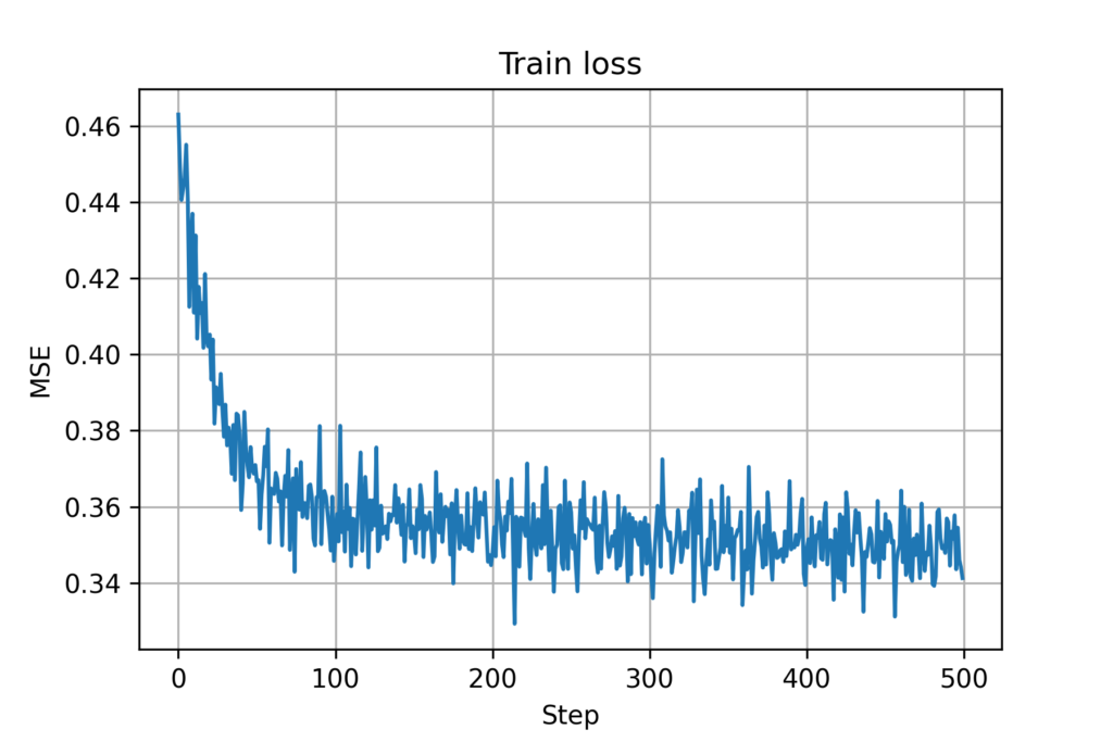
Figure 7. Training loss for GNN (with mobility)
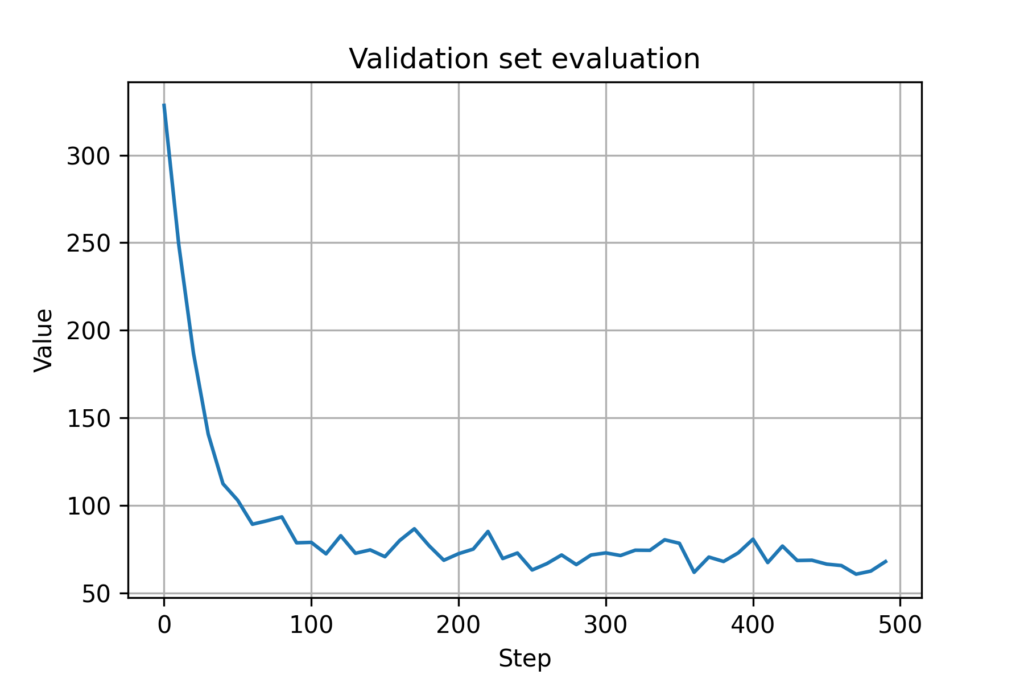
Figure 8. Validation cost for GNN (with mobility)
5.1-5.2 Collision Avoidance
Finally, we add another level of complexity to our simulation: collision avoidance. In simple terms, we consider a collision avoidance potential (28) which is then added to our cost function; thus, as agents get closer, the cost increases. We first create the Python function in the file $\p{networks}$ that computes the relative position difference between agents as:
def computeDifferences(u):
        #take input as: nSamples x tSamples x 2 x nAgents
    if len(u.shape) == 3:
        u = np.expand_dims(u, 1)
        hasTimeDim = False
    else:
        hasTimeDim = True
    nSamples = u.shape[0]
    tSamples = u.shape[1]
    nAgents = u.shape[3]
    uCol_x = u[:,:,0,:].reshape((nSamples, tSamples, nAgents, 1))
    uRow_x = u[:,:,0,:].reshape((nSamples, tSamples, 1, nAgents))
    uDiff_x = uCol_x - uRow_x
    uCol_y = u[:,:,1,:].reshape((nSamples, tSamples, nAgents, 1))
    uRow_y = u[:,:,1,:].reshape((nSamples, tSamples, 1, nAgents))
    uDiff_y = uCol_y - uRow_y
    uDistSq = uDiff_x ** 2 + uDiff_y ** 2
    uDiff_x = np.expand_dims(uDiff_x, 2)
    uDiff_y = np.expand_dims(uDiff_y, 2)
    uDiff = np.concatenate((uDiff_x, uDiff_y), 2)
    if not hasTimeDim:
        uDistSq = uDistSq.squeeze(1)
        uDiff = uDiff.squeeze(1)

    return uDiff, uDistSq
Based on (28)-(29), we create the python class $\p{OptimalControllerCollision}$ in the file $\p{consensus}$ for the optimal centralized controller with collision avoidance as:
class OptimalControllerCollision(ConsensusController):
    def __init__(self, sample_time=0.1, energy_weight=1):
        self.sample_time = sample_time
        self.energy_weight = energy_weight

    def __call__(self, gama, d0, pos, est_vel, biased_vel, step):

        ijDiffPos, ijDistSq = networks.computeDifferences(pos[:,step,:,:])
        gammaMask = (ijDistSq < (gama**2)).astype(ijDiffPos.dtype)
        ijDiffPos = ijDiffPos * np.expand_dims(gammaMask, 1)
        ijDistSqInv = ijDistSq.copy()
        ijDistSqInv[ijDistSq < 1e-9] = 1.
        ijDistSqInv = 1./ijDistSqInv
        ijDistSqInv[ijDistSq < 1e-9] = 0.
        ijDistSqInv = np.expand_dims(ijDistSqInv, 1)
        mean_biased_vel  = np.mean(biased_vel[:,step,:,:], axis=2)
        mean_biased_vel = np.expand_dims(mean_biased_vel, 2)
        accel = -(est_vel[:,step,:,:] - mean_biased_vel) / (self.sample_time * (1 + self.energy_weight)) + 1/self.sample_time/2*2* np.sum(ijDiffPos * (d0*d0*(ijDistSqInv ** 2) + d0*d0*ijDistSqInv), axis = 3)

        return accel
which takes agent positions as additional inputs. We create the python function $\p{simulateposcollision}$ in the class $\p{ConsensusSimulator}$ to simulate agent trajectories as:
    def simulate_pos_collision(self, wx, wy, degree, steps, controller: ConsensusController):

        ref_vel, est_vel = self.initial()
        bias = self.bias()
        x_pos = np.random.uniform(0, wx, (self.nSamples, 1, self.N))
        y_pos = np.random.uniform(0, wy, (self.nSamples, 1, self.N))
        pos = np.concatenate((x_pos, y_pos), axis = 1)
        ref_vels = np.zeros((self.nSamples, self.tSamples, 2, 1))
        est_vels = np.zeros((self.nSamples, self.tSamples, 2, self.N))
        biased_vels = np.zeros((self.nSamples, self.tSamples, 2, self.N))
        accels = np.zeros((self.nSamples, self.tSamples, 2, self.N))
        positions = np.zeros((self.nSamples, self.tSamples, 2, self.N))
        networkss = np.zeros((self.nSamples, self.tSamples, self.N, self.N))
        ref_vels[:,0,:,:] = ref_vel
        est_vels[:,0,:,:] = est_vel
        biased_vels[:,0,:,:] = bias + ref_vel
        positions[:,0,:,:] = pos
        accels[:,0,:,:] = controller(10, 2, positions, est_vels, biased_vels, 0)

        for i in range(self.nSamples):
            _, networkss[i,0,:,:] = networks.agent_communication_pos(positions[i,0,:,:], self.N, degree)
        this_accel = accels[:,0,:,:].copy()
        this_accel[accels[:,0,:,:] > self.max_agent_acceleration] = self.max_agent_acceleration
        this_accel[accels[:,0,:,:] < -self.max_agent_acceleration] = -self.max_agent_acceleration
        accels[:,0,:,:] = this_accel

        for step in range(1, steps):
            ref_accel = self.random_vector(self.ref_vel_delta, 1, self.nSamples)
            ref_vels[:,step,:,:] = ref_vels[:,step-1,:,:] + ref_accel * self.sample_time
            est_vels[:,step,:,:] = accels[:,step-1,:,:] * self.sample_time + est_vels[:,step-1,:,:]
            positions[:,step,:,:] = accels[:,step-1,:,:] * (self.sample_time ** 2)/2 + est_vels[:,step-1,:,:] * self.sample_time + positions[:,step-1,:,:]
            for i in range(self.nSamples):
                _, networkss[i,step,:,:] = networks.agent_communication_pos(positions[i,step,:,:], self.N, degree)
            biased_vels[:,step,:,:] = bias + ref_vels[:,step,:,:]
            accels[:,step,:,:] = controller(10, 2, positions, est_vels, biased_vels, step)
            this_accel = accels[:,step,:,:].copy()
            this_accel[accels[:,step,:,:] > self.max_agent_acceleration] = self.max_agent_acceleration
            this_accel[accels[:,step,:,:] < -self.max_agent_acceleration] = -self.max_agent_acceleration
            accels[:,step,:,:] = this_accel

        return networkss, positions, ref_vel, est_vel, est_vels, biased_vels, accels
To learn a GNN controller that mimics this optimal centralized controller, we now have an additional feature as the relative mass, and the file $\p{training}$ is modified as:
import torch
import numpy as np
import datetime
import networks
import copy

class TrainerFlocking(Trainer):

    def __init__(self, model, simulator, positions, ref_vel, est_vel, est_vels, biased_vels, accels, S, nEpochs, batchSize):

        super().__init__(model, simulator, positions, ref_vel, est_vel, est_vels, biased_vels, accels, S, nEpochs, batchSize)

    def train(self):

        nTrain = self.nTrain
        thisArchit = self.model.archit
        thisLoss = self.model.loss
        thisOptim = self.model.optim
        thisDevice = self.model.device
        epoch = 0
        pos_train = self.positions[0:self.nTrain]
        posDiff, posDistSq = networks.computeDifferences(pos_train)
        com_networks = copy.deepcopy(self.S[0:self.nTrain])
        com_networks = (np.abs(com_networks) > 1e-9).astype(self.positions.dtype)
        com_networks = np.expand_dims(com_networks, 2)
        posDiff = posDiff * com_networks
        statePos = np.sum(posDiff, axis = 4)
        xTrainAll = np.concatenate((self.est_vels[0:self.nTrain].copy(), self.biased_vels[0:self.nTrain].copy(), statePos), axis = 2)
        yTrainAll = self.accels[0:self.nTrain].copy()
        StrainAll = self.S[0:self.nTrain].copy()

        while epoch < self.nEpochs:

            randomPermutation = np.random.permutation(nTrain)
            idxEpoch = [int(i) for i in randomPermutation]

            batch = 0
            while batch < self.nBatches:

                thisBatchIndices = idxEpoch[self.batchIndex[batch] : self.batchIndex[batch+1]]
                xTrain = xTrainAll[thisBatchIndices]
                yTrain = yTrainAll[thisBatchIndices]
                Strain = StrainAll[thisBatchIndices]
                xTrain = torch.tensor(xTrain, device = thisDevice)
                Strain = torch.tensor(Strain, device = thisDevice)
                yTrain = torch.tensor(yTrain, device = thisDevice)
                startTime = datetime.datetime.now()
                thisArchit.zero_grad()
                yHatTrain = thisArchit(xTrain, Strain)
                lossValueTrain = thisLoss(yHatTrain, yTrain)
                lossValueTrain.backward()
                thisOptim.step()
                endTime = datetime.datetime.now()
                timeElapsed = abs(endTime - startTime).total_seconds()
                del xTrain
                del Strain
                del yTrain
                del lossValueTrain

                #\\\\\\\
                #\\\ VALIDATION
                #\\\\\\\

                if (epoch * self.nBatches + batch)

                    startTime = datetime.datetime.now()
                    ref_vel = self.ref_vel[220:240]
                    est_vel = self.est_vel[220:240]
                    position = self.positions[220:240]
                    _, _, est_vels_valid, biased_vels_valid, accels_valid = self.simulator.computeTrajectory_pos_collision(thisArchit, position, ref_vel, est_vel, 100)
                    accValid = self.simulator.cost(est_vels_valid, biased_vels_valid, accels_valid)
                    endTime = datetime.datetime.now()
                    timeElapsed = abs(endTime - startTime).total_seconds()

                    print("\t(E:
                            epoch+1, batch+1,
                            accValid,
                            timeElapsed), end = ' ')
                    print("[VALIDATION] \n", end = '')

                    if epoch == 0 and batch == 0:
                        bestScore = accValid
                        bestEpoch, bestBatch = epoch, batch
                        self.model.save(label = 'Best')
                        # Start the counter
                    else:
                        thisValidScore = accValid
                        if thisValidScore < bestScore:
                            bestScore = thisValidScore
                            bestEpoch, bestBatch = epoch, batch
                            print("\t=> New best achieved:
                            self.model.save(label = 'Best')
                    del ref_vel
                    del est_vel
                batch += 1
            epoch += 1

        self.model.save(label = 'Last')
        #################
        # TRAINING OVER #
        #################
        if self.nEpochs == 0:
            self.model.save(label = 'Best')
            self.model.save(label = 'Last')
            print("\nWARNING: No training. Best and Last models are the same.\n")
        self.model.load(label = 'Best')
        if self.nEpochs > 0:
            print("\t=> Best validation achieved (E:
                    bestEpoch + 1, bestBatch + 1, bestScore))
Here, for the validation, we similarly create the Python function $\p{computeTrajectoryposcollision}$ in the class $\p{ConsensusSimulator}$ as:
    def computeTrajectory_pos_collision(self, archit, position, ref_vel, est_vel, step):

        batchSize = est_vel.shape[0]
        nAgents = est_vel.shape[2]
        ref_vel = ref_vel.squeeze(2)
        architDevice = list(archit.parameters())[0].device
        est_vels = np.zeros((batchSize, step, 2, nAgents), dtype = np.float)
        ref_vels = np.zeros((batchSize, step, 2), dtype = np.float)
        positions = np.zeros((batchSize, step, 2, nAgents), dtype = np.float)
        biased_ref_vels = np.zeros((batchSize, step, 2, nAgents), dtype = np.float)
        bias = np.zeros((batchSize, step, 2, nAgents))
        accels = np.zeros((batchSize, step, 2, nAgents), dtype=np.float)
        states = np.zeros((batchSize, step, 6, nAgents), dtype=np.float)
        graphs = np.zeros((batchSize, step, nAgents, nAgents), dtype = np.float)
        com_networks = np.zeros((batchSize, step, nAgents, nAgents), dtype = np.float)
        est_vels[:,0,:,:] = est_vel.copy()
        ref_vels[:,0,:] = ref_vel.copy()
        bias[:,0,:,:] = np.random.normal(loc=0,scale=(4 * np.sqrt(2/np.pi)),size=(batchSize, 2, nAgents))
        ref_vel_temp = np.expand_dims(ref_vels[:,0,:], 2)
        biased_ref_vels[:,0,:,:] = ref_vel_temp + bias[:,0,:,:]
        positions[:,0,:,:] = position[:,0,:,:]

        for i in range(20):
            com_networks[i,0,:,:], graphs[i,0,:,:] = networks.agent_communication_pos(positions[i,0,:,:], nAgents, 2)

        for t in range(1, step):

            posDiff, posDistSq = networks.computeDifferences(positions[:,t-1,:,:])
            com_network = copy.deepcopy(com_networks[:,t-1,:,:])
            com_network = np.expand_dims(com_network, 1)
            posDiff = posDiff * com_network
            statePos = np.sum(posDiff, axis = 3)
            statePos = np.expand_dims(statePos, 1)
            thisbiased_ref_vels = np.expand_dims(biased_ref_vels[:,t-1,:,:], 1)
            thisest_vels = np.expand_dims(est_vels[:,t-1,:,:], 1)
            thisState = np.concatenate((thisest_vels, thisbiased_ref_vels, statePos), axis = 2)
            states[:,t-1,:,:] = thisState.squeeze(1)

            x = torch.tensor(states[:,0:t,:,:], device = architDevice)
            S = torch.tensor(graphs[:,0:t,:,:], device = architDevice)
            with torch.no_grad():
                thisaccels = archit(x, S)
            thisaccels = thisaccels.cpu().numpy()[:,-1,:,:]
            thisaccels[thisaccels > 3] = 3
            thisaccels[thisaccels < -3] = -3
            accels[:,t-1,:,:] = thisaccels
            est_vels[:,t,:,:] = accels[:,t-1,:,:] * 0.1 +est_vels[:,t-1,:,:]
            positions[:,t,:,:] = accels[:,t-1,:,:] * (0.1 ** 2)/2 + est_vels[:,t-1,:,:] * 0.1 + positions[:,t-1,:,:]
            ref_accel = np.random.normal(loc=0,scale=(self.ref_vel_delta * np.sqrt(2/np.pi)),size=(batchSize, 2))
            ref_vels[:,t,:] = ref_vels[:,t-1,:] + ref_accel * 0.1
            ref_vel_temp = np.expand_dims(ref_vels[:,t,:], 2)
            biased_ref_vels[:,t,:,:] = ref_vel_temp + bias[:,0,:,:]
            for i in range(20):
                com_networks[i,t,:,:], graphs[i,t,:,:] = networks.agent_communication_pos(positions[i,t,:,:], nAgents, 2)

        posDiff, posDistSq = networks.computeDifferences(positions[:,-1,:,:])
        com_network = copy.deepcopy(com_networks[:,-1,:,:])
        com_network = np.expand_dims(com_network, 1)
        posDiff = posDiff * com_network
        statePos = np.sum(posDiff, axis = 3)
        statePos = np.expand_dims(statePos, 1)
        thisbiased_ref_vels = np.expand_dims(biased_ref_vels[:,-1,:,:], 1)
        thisest_vels = np.expand_dims(est_vels[:,-1,:,:], 1)
        thisState = np.concatenate((thisest_vels, thisbiased_ref_vels, statePos), axis = 2)
        states[:,-1,:,:] = thisState.squeeze(1)
        x = torch.tensor(states, device = architDevice)
        S = torch.tensor(graphs, device = architDevice)
        with torch.no_grad():
            thisaccels = archit(x, S)
        thisaccels = thisaccels.cpu().numpy()[:,-1,:,:]
        thisaccels[thisaccels > 3] = 3
        thisaccels[thisaccels < -3] = -3
        accels[:,-1,:,:] = thisaccels

        return ref_vel, est_vel, est_vels, biased_ref_vels, accels
By aggregating all above modifications, we can perform the GNN training in the file $\p{main}$ as:
from importlib import reload
import numpy as np
import consensus
import networks
import os
import torch; torch.set_default_dtype(torch.float64)
import torch.nn as nn
import torch.optim as optim
import modules
import training
import model
import datetime
from copy import deepcopy
consensus = reload(consensus)
networks = reload(networks)

#
D = 2
K = 3
nSamples = 240
N = 100
step = 100
network = np.zeros((nSamples, N, N))
com_network = np.zeros((nSamples, step, N, N))

#
for i in range(nSamples):
    network[i,:,:], com_network[i,0,:,:] = networks.agent_communication(100, 200, N, D)
    for t in range(1, step):
        com_network[i,t,:,:] = deepcopy(com_network[i,0,:,:])

#
optimal_controller = consensus.OptimalController()
decentralized_controller = consensus.DistributedController(network, K)
simulator = consensus.ConsensusSimulator(N, nSamples)
optimal_controller_collision = consensus.OptimalControllerCollision()
networkss, positions, ref_vel, est_vel, est_vels, biased_vels, accels = simulator.simulate_pos_collision(100, 200, D, 100, optimal_controller_collision)

#
thisFilename = 'flockingGNN'
saveDirRoot = 'experiments'
saveDir = os.path.join(saveDirRoot, thisFilename)
today = datetime.datetime.now().strftime("
saveDir = saveDir + '-
# Create directory
if not os.path.exists(saveDir):
    os.makedirs(saveDir)

#   PyTorch seeds
torchState = torch.get_rng_state()
torchSeed = torch.initial_seed()
#   Numpy seeds
numpyState = np.random.RandomState().get_state()

nEpochs = 50 # Number of epochs
batchSize = 20 # Batch size
learningRate = 0.00025
beta1 = 0.9
beta2 = 0.999

hParamsLocalGNN = {