Lab 4: Resource Allocation in Wireless Communication Networks (10/28-11/15)
In a wireless communication system, information is transmitted in the form of an electromagnetic signal between a source and a destination. The feature that determines the quality of a communication link is the signal to noise ratio (SNR). In turn, the SNR of a channel is the result of multiplying the transmit power of the source by a propagation loss. This propagation loss is what we call a wireless channel. The problem of allocating resources in wireless communications is the problem of choosing transmit powers as a function of channel strength with the goal of optimizing some performance metric that is of interest to end users. Mathematically, the allocation of resources in wireless communications results in constrained optimization problems. Thus, in principle at least, all that is required to find an optimal allocation of resources is to find their solution. This is, however, impossible except in a few exceptional cases. In this lab we will explore the use of graph neural networks (GNNs) to find approximate solutions to the optimal allocation of resources in wireless communication systems.
1.1-1.2 Channel class and testing
First, let’s create a class to model a Channel and to contain its associated methods. The complete class can be found at Appendix at the bottom of this page, but let’s show the process of constructing the class. Let’s start with the initialization and the first method:
import numpy as np
import matplotlib.pyplot as plt
import torch
from scipy.spatial import distance_matrix
from tqdm import tqdm
from typing import List, Union, Tuple
import torch
from torch import nn
class Channel(object):
def __init__(self, d0, gamma, s, N0):
"""
Object for modeling a channel
Args:
d0: Reference distance.
gamma: Path loss exponent.
s: Fading energy.
N0: Noise floor.
"""
self.d0 = d0
self.gamma = gamma
self.s = s
self.N0 = N0
def pathloss(self, d):
"""
Question 1.1
Calculate simplified path-loss model.
Args:
d: The distance. Can be a matrix - this is an elementwise operation.
Returns: Pathloss value.
"""
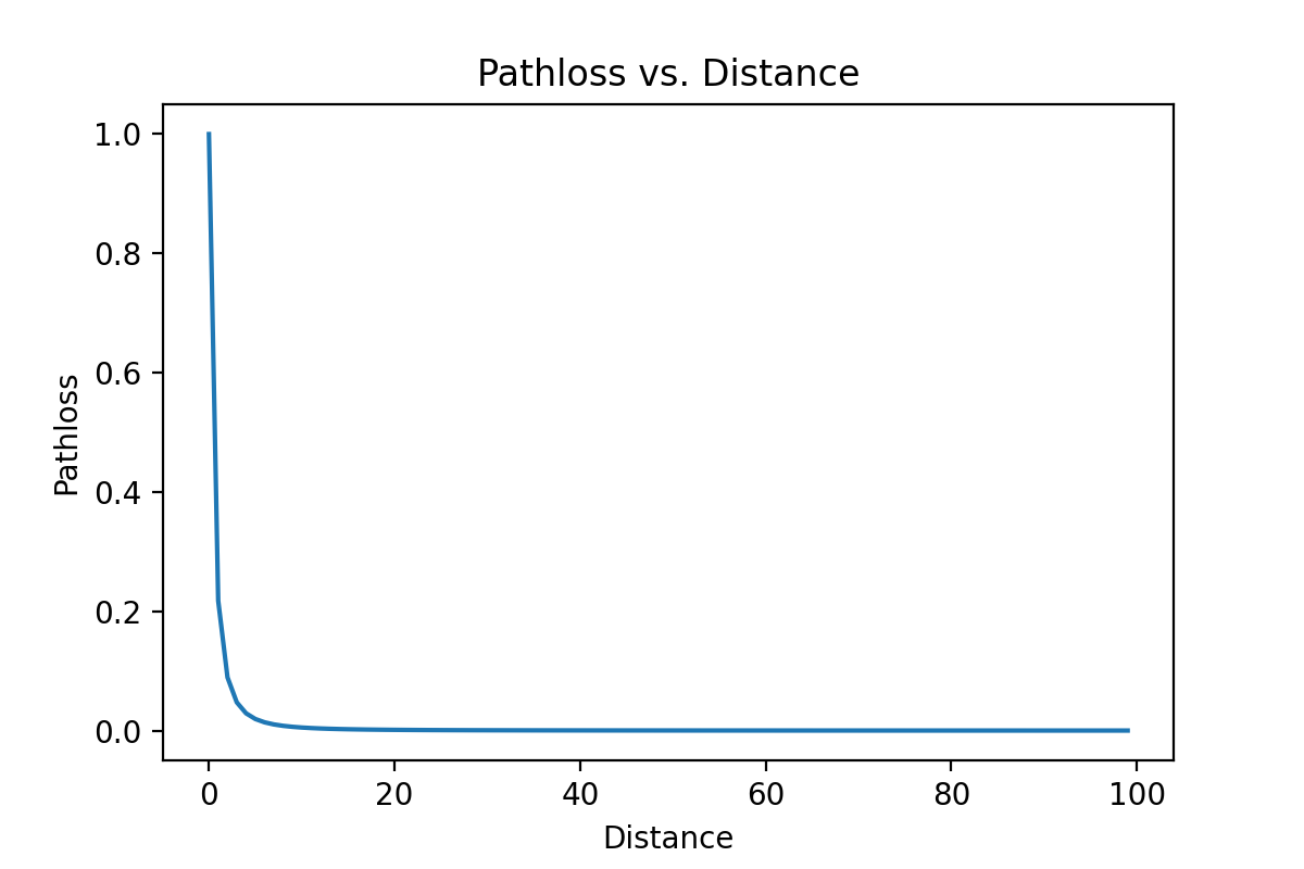
return (self.d0 / d) ** self.gamma
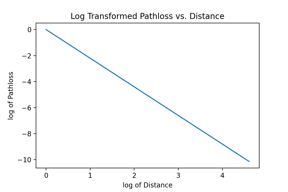
Test and plot with distance ranging from $1m$ to $100m$: Plot the pathloss with linear and logarithmic scale.
# Create distances from 1 - 100
dist = np.arange(1,101)

# Create channel object with values from Figure 1
channel = Channel(1, 2.2, 2, 1e-6)

# Calculate 100 pathloss values
Exp_h = channel.pathloss(dist)

# Plot in linear scale
plt.figure()
plt.plot(Exp_h)
plt.ylabel('Pathloss')
plt.xlabel('Distance')
plt.title("Pathloss vs. Distance")
plt.savefig('PathlossLin.png', dpi = 200)
plt.show()

# Plot in logarithmic scale
plt.figure()
plt.plot(np.log(dist), np.log(Exp_h))
plt.ylabel('log of Pathloss')
plt.xlabel('log of Distance')
plt.title("Log Transformed Pathloss vs. Distance")
plt.savefig('PathlossLog.png', dpi = 200)
plt.show()
1.3-1.4 Fading channel class and testing
Next, we build the method for computing the fading channel model:
def fading_channel(self,d, Q):
"""
Question 1.3
Calculate fading channel model.
Args:
d: The distance. Can be a matrix - this is an elementwise operation.
Q: Number of random samples.
Returns: Q fading channel realizations
"""
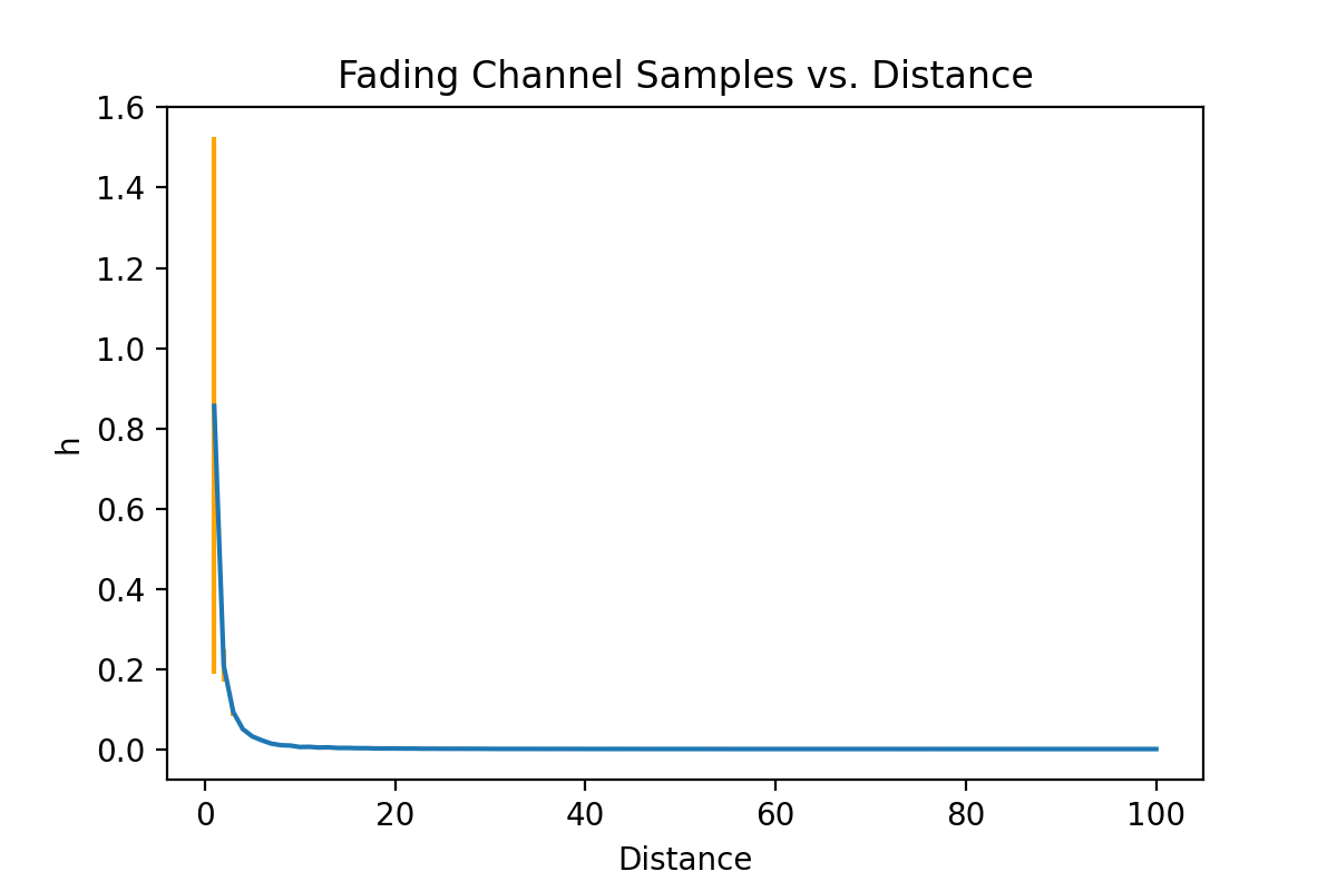
Exp_h = (self.d0 / d) ** self.gamma
h_til = np.random.exponential(self.s, size=(1, Q))
h = Exp_h * h_til / self.s
return h
Test and plot with distance ranging from $1m$ to $100m$:
# 100 channel realizations
Q = 100

# Initialize a matrix to store results
h_sim = np.zeros((100, Q))

# Consider distances from 1 - 100 meters
# and compute 100 realizations of at each
for d in dist:
    h_sim[d-1,:] = channel.fading_channel(d, 100)

# Calculate mean and var of these realizations
h_mean = np.mean(h_sim, axis = 1)
h_var = np.var(h_sim, axis = 1)

# Plot
plt.figure()
plt.errorbar(dist, h_mean, h_var, ecolor='orange')
plt.ylabel('h')
plt.xlabel('Distance')
plt.title("Fading Channel Samples vs. Distance")
plt.savefig('FadingChannelSamples.png', dpi = 200)
plt.show()
1.5-1.6 Capacity method and testing
Last, we add the method for modeling a fading capacity channel:
def build_fading_capacity_channel(self, h, p):
"""
Question 1.5
Calculate fading capacity channel model.
Args:
h: Fading channel realizations (of length Q).
p: Power values (of length Q).
Returns: Q channel capacity values
"""
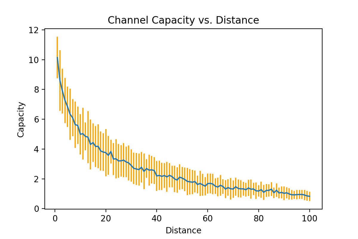
return np.log(1 + h * p / self.N0)
Test and plot with distance ranging from $1m$ to $100m$:
# Using h_sim from 1.4, calculate Q channel capacity values
cap = channel.build_fading_capacity_channel(h_sim, 0.05)

# Calculate mean and var of these realizations
cap_mean = np.mean(cap, axis = 1)
cap_var = np.var(cap, axis = 1)

# Plot
plt.figure()
plt.errorbar(dist, cap_mean, cap_var, ecolor="orange")
plt.ylabel('Capacity')
plt.xlabel('Distance')
plt.title('Channel Capacity vs. Distance')
plt.savefig('ChannelCapacities.png', dpi = 200)
plt.show()
2.1 Transmitter and Receiver Positioning
We define a class to model the Wireless Network, which takes as input information on the area, the number of transmitter/receivers, and channel information. The complete class is provided in the Appendix at the bottom of the page.
class WirelessNetwork(object):
    def __init__(self, wx, wy, wc, n, d0, gamma, s, N0):
        """
        Object for modeling a Wireless Network

        Args:
            wx: Length of area.
            wy: Width of area.
            wc: Max distances of receiver from its transmitter.
            n: Number of transmitters/receivers.
            d0: Refernce distance.
            gamma: Pathloss exponent.
            s: Fading energy.
            N0: Noise floor.
        """
        self.wx = wx
        self.wy = wy
        self.wc = wc
        self.n = n

        # Determines transmitter and receiver positions
        self.t_pos, self.r_pos = self.determine_positions()

        # Calculate distance matrix using scipy.spatial method
        self.dist_mat = distance_matrix(self.t_pos, self.r_pos)

        self.d0 = d0
        self.gamma = gamma
        self.s = s
        self.N0 = N0

        # Creates a channel with the given parameters
        self.channel = Channel(self.d0, self.gamma, self.s, self.N0)
To this class, we add a method to determine initial positions:
    def determine_positions(self):
        """
        Question 2.1
        Calculate positions of transmitters and receivers

        Returns: transmitter positions, receiver positions
        """
        # Calculate transmitter positions
        t_x_pos = np.random.uniform(0, self.wx, (self.n, 1))
        t_y_pos = np.random.uniform(0, self.wy, (self.n, 1))
        t_pos = np.hstack((t_x_pos, t_y_pos))

        # Calculate receiver positions
        r_distance = np.random.uniform(0, self.wc, (self.n, 1))
        r_angle = np.random.uniform(0, 2 * np.pi, (self.n, 1))
        r_rel_pos = r_distance * np.hstack((np.cos(r_angle), np.sin(r_angle)))
        r_pos = t_pos + r_rel_pos
        return t_pos, r_pos
2.2 Pathloss
To compute the pathloss matrix, we can use our pathloss method from Channel:
    def generate_pathloss_matrix(self):
        """
        Question 2.2
        Calculates pathloss matrix

        Returns: pathloss matrix
        """
        return self.channel.pathloss(self.dist_mat)
2.3 Fading
Similarly, to compute the interference matrix, we can use our fading channel method from Channel:
    def generate_interference_graph(self, Q):
        """
        Question 2.3
        Calculates interference graph

        Returns: interference graph
        """
        return self.channel.fading_channel(self.dist_mat, Q)
2.4 Channel Capacity
Lastly, we compute the capacity for each transmitter through the equations provided in the lab write-up:
    def generate_channel_capacity(self, p, H):
        """
        Question 2.4
        Calculates capacity for each transmitter

        Returns: capacity for each transmitter
        """
        num = torch.diagonal(H, dim1=-2, dim2=-1) * p
        den = H.matmul(p.unsqueeze(-1)).squeeze() - num + self.N0
        return torch.log(1 + num / den)
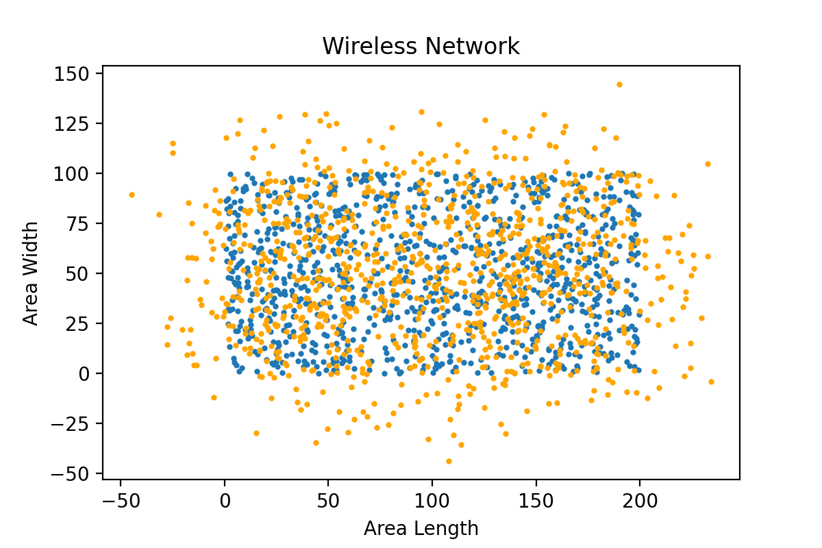
To generate a plot of the Wireless Network, we add a method to the WirelessNetwork object, initialize an object with the given parameters, and call upon the plot method:
    def plot_network(self):
        """
        Creates a plot of the given Wireless Network
        """
        plt.scatter(self.t_pos[:,0], self.t_pos[:,1], s = 4, label = "Transmitters")
        plt.scatter(self.r_pos[:,0], self.r_pos[:,1], s = 4, label = "Receivers", c = "orange")
        plt.xlabel("Area Length")
        plt.ylabel("Area Width")
        plt.title("Wireless Network")
        plt.savefig('WirelessNetwork.png', dpi = 200)
        plt.legend()
        return plt.show()
d0 = 1
gamma = 2.2
s = 2
N0 = 1e-6
rho = 0.05
wc = 50
wx = 200
wy = 100
n = int(rho * wx * wy)

WirelessNetwork(wx, wy, 50, n, d0, gamma, s, N0).plot_network()
3.1 Unconstrained training
The input to GNN in this application is a graph with edges generated from a random distribution. Each training iteration we need to generate a random graph structure. Therefore, we first construct a generator class
class Generator:
    def __init__(self, n, wx, wy, wc, d0=1, gamma=2.2, s=2, N0=1, device="cpu", batch_size=64, random=False):
        # Save the configurations for the Wireless Network
        self.n = n
        self.wx = wx
        self.wy = wy
        self.wc = wc

        # Save the Channel configurations
        self.d0 = d0
        self.gamma = gamma
        self.s = s
        self.N0 = N0

        # Training configurations
        self.device = device
        self.batch_size = batch_size

        # True if pathloss should change at random
        self.random = random

        self.train = None
        self.test = None

        # Generate a Wireless Network and pathloss matrix
        self.network = WirelessNetwork(self.wx, self.wy, self.wc, self.n, self.d0,
                                       self.gamma, self.s, self.N0)
        self.H1 = self.network.generate_pathloss_matrix()

    def __next__(self):
        if self.random:
            # Generate a new random network
            self.network = WirelessNetwork(self.wx, self.wy, self.wc, self.n, self.d0,
                                       self.gamma, self.s, self.N0)
            self.H1 = self.network.generate_pathloss_matrix()
        H2 = np.random.exponential(self.s, (self.batch_size, self.n, self.n))

        # Generate random channel matrix
        H = self.H1 * H2

        # Normalization of the channel matrix
        eigenvalues, _ = np.linalg.eig(H)
        S = H / np.max(eigenvalues.real)

        # Put onto device
        H = torch.from_numpy(H).to(torch.float).to(self.device)
        S = torch.from_numpy(S).to(torch.float).to(self.device)
        return H, S, self.network
Next, we need to define a $\p{train}$ and $\p{test}$ function to help evaluate the strategy. For the $\p{train}$ function, we take the GNN model, the update rules, and the network generator as inputs.
def train(model, update, generator, iterations):
    pbar = tqdm(range(iterations), desc=f"Training for n={generator.n}")
    for i in pbar:
        # For each iteration, generate a new random channel matrix
        H, S, network = next(generator)
        # Get the corresponding allocation strategy
        p = model(S)

        # Calculate the capacity as the performance under this allocation strategy
        c = network.generate_channel_capacity(p, H)
        # Update the parameters of the model
        update(p, c)
        pbar.set_postfix({'Capacity Mean': f" {c.mean().item():.3e}",
                          'Capacity Var': f" {c.var().item():.3e}",
                          'Power Mean': f" {p.mean().item():.3f}",
                          'Power Var': f" {p.var().item():.3f}"})
For the $\p{test}$ function, we do not need to update the model but just verify with random generated networks and output the performance.
def test(model: Callable[[torch.Tensor], torch.Tensor], generator: Generator, iterations=100):
    powers = []
    capacities = []
    loss = []
    for i in tqdm(range(iterations), desc=f"Test for n={generator.n}"):
        # For each iteration, generate a new random channel matrix
        H, S, network = next(generator)
        # Get the corresponding allocation strategy
        p = model(S)
        # Calculate the capacity as the performance under this allocation strategy
        c = network.generate_channel_capacity(p, H)

        # Save the loss, capacities, and powers
        loss.append(-c.mean().item() + mu_unconstrained * p.mean().item())
        capacities.append(c.mean().item())
        powers.append(p.mean().item())
    print()
    print("Testing Results:")
    print(f"\tLoss mean: {np.mean(loss):.4f}, variance {np.var(loss):.4f}"
          f"| Capacity mean: {np.mean(capacities):.4e}, variance {np.var(capacities):.4e}"
          f"| Power mean: {np.mean(powers):.4f}, variance {np.var(powers):.4f}")
With the GSO changing each iteration, we also need to define a new GNN class to take graph signal $\bbx$ and $\bbH$ both as inputs.
We begin with define the graph filter class in the $\p{graph.py}$ file.
class GraphFilter(nn.Module):
    def __init__(self, k: int, f_in=1, f_out=1, f_edge=1):
        """
        A graph filter layer.
        Args:
            gso: The graph shift operator.
            k: The number of filter taps.
            f_in: The number of input features.
            f_out: The number of output features.
        """
        super().__init__()
        self.k = k
        self.f_in = f_in
        self.f_out = f_out
        self.f_edge = f_edge

        self.weight = nn.Parameter(torch.ones(self.f_out, self.f_edge, self.k, self.f_in))
        self.bias = nn.Parameter(torch.zeros(self.f_out, 1))
        torch.nn.init.normal_(self.weight, 0.3, 0.1)
        torch.nn.init.zeros_(self.bias)

    def to(self, *args, **kwargs):
        # Only the filter taps and the weights are registered as
        # parameters, so we need to move gsos ourselves.

        self.weight = self.gso.to(*args, **kwargs)
        self.bias = self.gso.to(*args, **kwargs)
        return self

    def forward(self, x: torch.Tensor, S: torch.Tensor):
        batch_size = x.shape[0]

        B = batch_size
        E = self.f_edge
        F = self.f_out
        G = self.f_in
        N = S.shape[-1]  # number of nodes
        K = self.k   # number of filter taps

        h = self.weight
        b = self.bias

        # Now, we have x in B x G x N and S in E x N x N, and we want to come up
        # with matrix multiplication that yields z = x * S with shape
        # B x E x K x G x N.
        # For this, we first add the corresponding dimensions
        x = x.reshape([B, 1, G, N])
        S = S.reshape([batch_size, E, N, N])
        z = x.reshape([B, 1, 1, G, N]).repeat(1, E, 1, 1, 1)  # This is for k = 0
        # We need to repeat along the E dimension, because for k=0, S_{e} = I for
        # all e, and therefore, the same signal values have to be used along all
        # edge feature dimensions.
        for k in range(1, K):
            x = torch.matmul(x, S)  # B x E x G x N
            xS = x.reshape([B, E, 1, G, N])  # B x E x 1 x G x N
            z = torch.cat((z, xS), dim=2)  # B x E x k x G x N
        # This output z is of size B x E x K x G x N
        # Now we have the x*S_{e}^{k} product, and we need to multiply with the
        # filter taps.
        # We multiply z on the left, and h on the right, the output is to be
        # B x N x F (the multiplication is not along the N dimension), so we reshape
        # z to be B x N x E x K x G and reshape it to B x N x EKG (remember we
        # always reshape the last dimensions), and then make h be E x K x G x F and
        # reshape it to EKG x F, and then multiply
        y = torch.matmul(z.permute(0, 4, 1, 2, 3).reshape([B, N, E * K * G]),
                         h.reshape([F, E * K * G]).permute(1, 0)).permute(0, 2, 1)
        # And permute again to bring it from B x N x F to B x F x N.
        # Finally, add the bias
        if b is not None:
            y = y + b
        return y
Based on the above definitions, we can further define the GNN structure.
class GraphNeuralNetwork(nn.Module):
    def __init__(self,
                 ks: Union[List[int], Tuple[int]] = (5,),
                 fs: Union[List[int], Tuple[int]] = (1, 1)):
        """
        An L-layer graph neural network. Uses ReLU activation for each layer except the last, which has no activation.

        Args:
            gso: The graph shift operator.
            ks: [K_1,...,K_L]. On ith layer, K_{i} is the number of filter taps.
            fs: [F_1,...,F_L]. On ith layer, F_{i} and F_{i+1} are the number of input and output features,
             respectively.
        """
        super().__init__()
        self.n_layers = len(ks)

        self.layers = []
        for i in range(self.n_layers):
            f_in = fs[i]
            f_out = fs[i + 1]
            k = ks[i]
            gfl = GraphFilter(k, f_in, f_out)
            activation = torch.nn.ReLU() if i < self.n_layers - 1 else torch.nn.Identity()
            self.layers += [gfl, activation]
            self.add_module(f"gfl{i}", gfl)
            self.add_module(f"activation{i}", activation)

    def forward(self, x, S):
        for i, layer in enumerate(self.layers):
            x = layer(x, S) if i
        return x
Then we customize the GNN model and define a class:
class Model(torch.nn.Module):
    def __init__(self, gnn):
        super().__init__()
        self.gnn = gnn

    def forward(self, S):
        batch_size = S.shape[0]
        n = S.shape[1]
        p0 = torch.ones(batch_size, n, device=device)
        p = self.gnn(p0, S).abs()
        return torch.squeeze(p)
We need to specify the loss function of this unconstrained learning as:
\begin{align}\label{eqn_unconstrained_loss}
\sum\limits_{i=1}^n \mathbb{E}[f_i(\Phi(\bbH,\bbA), \bbH)] – \mu_i\mathbb{E}[\Phi_i(\bbH,\bbA)].
\end{align}
Because of the unknown of distribution $m(\bbH)$, the expectation cannot be calculated explicily. We approximate the expectation value with the average of a batch of data. As $n$ is determined here, we use the mean value as evaluations rather than sum values.
mu_unconstrained = 0.01  ## importance weights set as 0.01
step_size = 0.01
device = "cuda:0" if torch.cuda.is_available() else "cpu"
unconstrained = Model(GraphNeuralNetwork([5, 5, 5], [1, 8, 4, 1]).to(device)) #GNN build-up
optimizer = torch.optim.Adam(unconstrained.parameters(), step_size)

def update_unconstrained(p, c):
    global mu, optimizer
    optimizer.zero_grad()
    objective = -c.mean() + mu_unconstrained * p.mean()  # Specify loss function
    objective.backward()
    optimizer.step()
With the wireless network and GNN structured, we can implement the wireless network generation function and build up the networks. The input dimensions are $w_x=80m$, $w_y=40m$, $w_c=20m$. The number of nodes $n$ is calculated with $\rho=\frac{n}{w_x w_y}=0.005$. The wireless network then can be generated as:
N0 = 1e-6
train_iterations = 200
test_iterations = 100
batch_size = 100

device = "cuda:0" if torch.cuda.is_available() else "cpu"

generator_small = Generator(160, 80, 40, 20, device=device, N0=N0, batch_size=batch_size)
We can then input the unconstrained learning GNN model, the updating rule and the generator defined above to train and test the GNN.
train(unconstrained, update_unconstrained, generator_small, train_iterations)
test(unconstrained, generator_small, test_iterations)
| Avg. Loss | Avg. Capacity | Avg. Power |
|---|---|---|
| -0.3321 | 0.3335 | 0.1350 |
3.2 Stability
We verify the trained GNN in 3.1 by testing on 100 other networks with the same parameters. Here other networks indicate different positioning of transmitters and receivers. We realize this by setting the input parameter $\p{random}$ of function $\p{wireless.Generator}$ as $\p{true}$. This makes the generator produces different $160-$node wireless networks with a number of $\p{batch\_size}$. The generator therefore needs to be called as:
generator_random = Generator(160, 80, 40, 20, device=device, N0=N0, batch_size=batch_size, random=True)
test(unconstrained, generator_random, test_iterations)
| Avg. Loss | Avg. Capacity | Avg. Power |
|---|---|---|
| -0.1893 | 0.1906 | 0.1372 |
3.3 Transference
We verify the transference by generating another set of larger networks. With $\rho$ keeping the same and $w_x=120m$, $w_y=60m$, $w_c=30m$, the number of nodes in the newly generated setting is $n=360$.
generator_large = Generator(360, 120, 60, 30, device=device, N0=N0, batch_size=batch_size, random=True)
test(unconstrained, generator_large, test_iterations)
| Avg. Loss | Avg. Capacity | Avg. Power |
|---|---|---|
| -0.1263 | 0.1276 | 0.1337 |
4.1 Constrained training
Compared with the unconstrained training, the difference for constrained training mainly lies in the updating process. Instead of operating SGD once, we need to carry out gradient ascent on the primal variable $\bbA$ as equation (26) and gradient descent on the dual variable $\mu$ as equation (25).
def update_constrained(p, c):
    global mu, optimizer
    optimizer.zero_grad()

    # primal step
    (mu.unsqueeze(0) * (p - pmax) - c).mean().backward()
    optimizer.step()
    # dual step
    with torch.no_grad():
        mu = torch.relu(mu + dual_step * torch.mean((p - pmax), 0))
Then we need to set up the parameters needed in this setting, we set the primal update stepsize as $0.01$ and dual stepsize as $0.001$. The weight vector $\mathbf{\mu}$ is initialized to be all zero vector.
primal_step = 0.01
dual_step = 0.001

mu = torch.zeros(generator_small.n, device=device)
constrained = Model(GraphNeuralNetwork([5, 5, 5], [1, 8, 4, 1]).to(device))
optimizer = torch.optim.Adam(constrained.parameters(), primal_step)
The implementation of constrained learning is similar to the steps of unconstrained learning:
train(constrained, update_constrained, generator_small, train_iterations)
test(constrained, generator_small, test_iterations)
| Avg. Loss | Avg. Capacity | Avg. Power |
|---|---|---|
| -0.3329 | 0.3330 | 0.0134 |
4.2 Stability
Run the test script with the random network generator:
test(constrained, generator_random, test_iterations)
| Avg. Loss | Avg. Capacity | Avg. Power |
|---|---|---|
| -0.1818 | 0.1819 | 0.0142 |
4.3 Transference
Run the test script with the large network generator:
test(constrained, generator_large, test_iterations)
| Avg. Loss | Avg. Capacity | Avg. Power |
|---|---|---|
| -0.1218 | 0.1201 | 0.0107 |
Appendix
import numpy as np
import matplotlib.pyplot as plt
import torch
from scipy.spatial import distance_matrix
from tqdm import tqdm

class Channel(object):
    def __init__(self, d0, gamma, s, N0):
        """
        Object for modeling a channel

        Args:
            d0: Reference distance.
            gamma: Path loss exponent.
            s: Fading energy.
            N0: Noise floor.
        """
        self.d0 = d0
        self.gamma = gamma
        self.s = s
        self.N0 = N0

    def pathloss(self, d):
        """
        Question 1.1
        Calculate simplified path-loss model.

        Args:
            d: The distance. Can be a matrix - this is an elementwise operation.

        Returns: Pathloss value.
        """
        return (self.d0 / d) ** self.gamma

    def fading_channel(self,d, Q):
        """
        Question 1.3
        Calculate fading channel model.

        Args:
            d: The distance. Can be a matrix - this is an elementwise operation.
            Q: Number of random samples.

        Returns: Q fading channel realizations
        """
        Exp_h = (self.d0 / d) ** self.gamma
        h_til = np.random.exponential(self.s, size=(1, Q))
        h = Exp_h * h_til / self.s
        return h

    def build_fading_capacity_channel(self, h, p):
        """
        Question 1.5
        Calculate fading capacity channel model.

        Args:
            h: Fading channel realizations (of length Q).
            p: Power values (of length Q).

        Returns: Q channel capacity values
        """
        return np.log(1 + h * p / self.N0)
class WirelessNetwork(object):
    def __init__(self, wx, wy, wc, n, d0, gamma, s, N0):
        """
        Object for modeling a Wireless Network

        Args:
            wx: Length of area.
            wy: Width of area.
            wc: Max distances of receiver from its transmitter.
            n: Number of transmitters/receivers.
            d0: Refernce distance.
            gamma: Pathloss exponent.
            s: Fading energy.
            N0: Noise floor.
        """
        self.wx = wx
        self.wy = wy
        self.wc = wc
        self.n = n

        # Determines transmitter and receiver positions
        self.t_pos, self.r_pos = self.determine_positions()

        # Calculate distance matrix using scipy.spatial method
        self.dist_mat = distance_matrix(self.t_pos, self.r_pos)

        self.d0 = d0
        self.gamma = gamma
        self.s = s
        self.N0 = N0

        # Creates a channel with the given parameters
        self.channel = Channel(self.d0, self.gamma, self.s, self.N0)

    def determine_positions(self):
        """
        Question 2.1
        Calculate positions of transmitters and receivers

        Returns: transmitter positions, receiver positions
        """
        # Calculate transmitter positions
        t_x_pos = np.random.uniform(0, self.wx, (self.n, 1))
        t_y_pos = np.random.uniform(0, self.wy, (self.n, 1))
        t_pos = np.hstack((t_x_pos, t_y_pos))

        # Calculate receiver positions
        r_distance = np.random.uniform(0, self.wc, (self.n, 1))
        r_angle = np.random.uniform(0, 2 * np.pi, (self.n, 1))
        r_rel_pos = r_distance * np.hstack((np.cos(r_angle), np.sin(r_angle)))
        r_pos = t_pos + r_rel_pos
        return t_pos, r_pos

    def generate_pathloss_matrix(self):
        """
        Question 2.2
        Calculates pathloss matrix

        Returns: pathloss matrix
        """
        return self.channel.pathloss(self.dist_mat)

    def generate_interference_graph(self, Q):
        """
        Question 2.3
        Calculates interference graph

        Returns: interference graph
        """
        return self.channel.fading_channel(self.dist_mat, Q)

    def generate_channel_capacity(self, p, H):
        """
        Question 2.4
        Calculates capacity for each transmitter

        Returns: capacity for each transmitter
        """
        num = torch.diagonal(H, dim1=-2, dim2=-1) * p
        den = H.matmul(p.unsqueeze(-1)).squeeze() - num + self.N0
        return torch.log(1 + num / den)

    def plot_network(self):
        """
        Creates a plot of the given Wireless Network
        """
        plt.scatter(self.t_pos[:,0], self.t_pos[:,1], s = 4, label = "Transmitters")
        plt.scatter(self.r_pos[:,0], self.r_pos[:,1], s = 4, label = "Receivers", c = "orange")
        plt.xlabel("Area Length")
        plt.ylabel("Area Width")
        plt.title("Wireless Network")
        plt.savefig('WirelessNetwork.png', dpi = 200)
        plt.legend()
        return plt.show()