Using linear parameterizations can be seen to fail even when the model is linear if we don’t have enough data. In this post, we will see that neural networks (NN) can success in learning non-linear models, but this is only true if we have sufficient data.
In this post we will work with the simplest NN – a two layer fully connected NN – that can be express by the following equation,
\begin{equation}\label{eqn_nn}
\hby \ =\ \bbH_2 \bbz
\ =\ \bbH_2 \Big (\, \sigma \big(\,\bbH_1\bbx\,\big) \,\Big) ,
\end{equation}
where the matrix $\bbH_1$ is $h \times n$ and the matrix $\bbH_2$ is $m \times h$ and $\sigma$ is a point wise non-linearity. The scalar constant $h$ is the number of hidden units, $n$ is the size of the input vector, and $m$ is the size of the output vector.
Neural Networks with Sufficient Data
For this section we will construct a non-linear model as a minor variation of a linear model. In order to create a non-linear model, we will compose the absolute value function,
\begin{align}\label{eqn_non_linear_model}
\bby=|\bbA \bbx + \bbw|,
\end{align}
where observations $\bbx\in\reals^n$ and noise $\bbw \in \reals^m$ are drawn from independent multivariate Gaussian distributions with zero mean and energy $\mbE[||\bbx||^2]=\mbE[||\bbw||^2]=1/2$. Matrix $A \in \reals^{m \times n}$ is a matrix whose components are iid drawn from a Bernoulli distribution of parameters $1/m$.
Learning for us will be to succeed at minimizing an empirical risk minimization. The loss function that we will use in this case is the mean square error (MSE),
\begin{align}\label{eqn_ERM_nn}
\bbH^* =\ \arg \min_{\bbH\in\reals^{m\times n}}
\frac{1}{Q} \sum_{q=1}^Q \,
\frac{1}{2} \,
\left \| \,
\bby_q-
\bbH_2\Big(\sigma\big(\bbH_1\bbx_q\big)\Big)
\,\right \|^2_2 .
\end{align}
We will tackle this problem by using stochastic gradient descent, and Pytorch as the tool that computes the automatic differentiation for us. We will plot the loss on two sets, one that we will use for training and another one that we will keep for testing the performance of the NN on unseen data. This approach of separating data helps us as a means of assessing the generalization abilities on unseen data.

In figure (1) we plotted the MSE for a two-layer NN parametrized in Pytorch with $h=100$ hidden units. We have used $Q=1000$ samples for the training test and $100$ samples for the testing set. Figure (1) shows how our NN can successfully predict unseen samples by decreasing the MSE in the testing set. In this case, the amount of data that we have allows the NN to decrease the MSE of both the training and the testing sets, which shows that the NN is able to successfully learn the model.
Neural Networks with Insufficient Data
To visualize the effect of not having enough data, consider again the problem of the non-linear model \eqref{eqn_non_linear_model}. Consider also using the same NN as before, but now we will restrict ourselves to a small number of samples. Instead of having the $Q=1000$, we will only have $Q=50$ samples. This means that our dataset is 20 times smaller than the one in the previous section.
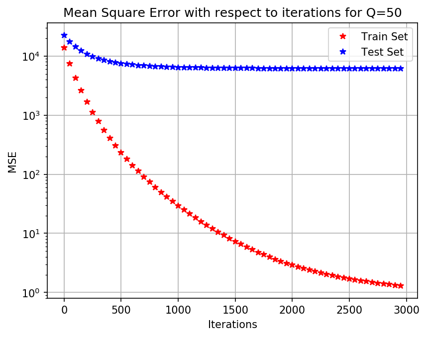
Figure (2) shows how the NN is not able to decrease the MSE on the test set, in this case the error is at least $100$ times larger than in the case of (1). With this numerical example we show that NN may be a correct parameterization to use, albeit they do suffer from lack of data, just as the linear parameterization.
In this easy numerical example we showed that NN become handy when the model is either not known or it is difficult to use. The results show how NN can successfully outperform the linear parameterizations on non-linear models. However, when data is not sufficient, both NN and linear parameterizations tend to increase the error in the testing set, failing to generalize on un-seen data. The results are conclusive, NN are not magical, they do not work unless they are provided with the sufficient amount of data.
Code Links
Implementations of the training loop described in this document, can be found in the folder code\_non\_linear\_loops.zip. This folder contains the following files:
$\p{main\_data.py}$: This is the main script, where parameters are given and the learning loop is implemented.
$\p{achitectures.py}$: This is the script in which the two-layer neural network class is defined. In short, $\p{\_\_init\_\_}$ is called when the class $\p{TwoLayerNN}$ is instanced and $\p{forward}$ is a method which computes the output of the NN. Notice that we have chosen $\p{ReLU}$ as the point wise non-linearity.
$\p{data.py}$: This is the script where the data is created, the data follows the non-linear model given in $\eqref{eqn_non_linear_model}$.
$\p{plot\_results.py}$: In this script the plots are done, both figures (1) and (2) where obtained with this script.